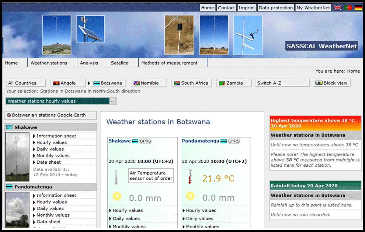
Figure 1
Visualisation of AWS data via the SASSCAL Weathernet.
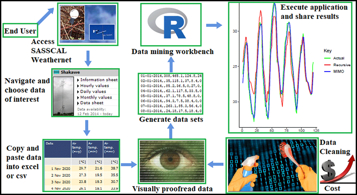
Figure 2
Manually extracting data from the SASSCAL Weathernet. This process is costly, time consuming and error-prone.
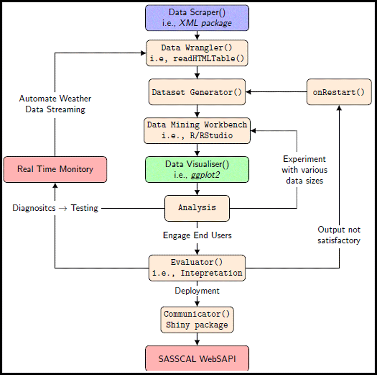
Figure 3
Workflow of the SASSCAL WebSAPI.
Table 1
R packages proposed in this work.
| PACKAGE | DESCRIPTION |
|---|---|
| rvest (Wickham & Wickham 2016) | web scraping |
| Xml2 (Lang & Lang 2015) | XML document processing |
| stringr (Wickham & Wickham 2019) | data cleaning and preparation |
| ggplot (Wickham 2011) | visualisation of graphics |
| shiny (Chang et al. 2015) | dashboard design |
| leaflet (Graul & Graul 2016) | reactive maps |
| dygraphs (Vanderkam et al. 2015) | time-series data and interactivity |
| data.table (Dowle et al. 2019) | tables and data munging |
| flexdashboard (Allaire 2017) | shiny dashboard design |
Algorithm 1
Visualise the AWSs of a given country.
| 1 | c←dataframe(w, x, y, z) |
| 2 | leaflet(data = c) %>% |
| 3 | addTiles() %>% |
| 4 | setMaxBounds(x1, y2, x2, y2) %>% |
| 5 | addMarkers(∼ long,∼ lat, label= ∼ name) |
Algorithm 2
Data scraper.
| 1 | AWS_ID_Getter← function(AWS) { |
| 2 | V = c(“x”, “value”); parent = emptyenv() |
| 3 | assign_hash ← Vectorize(assign, vectorize.args = V) |
| 4 | get_hash ← Vectorize(get, vectorize.args = “x”) |
| 5 | exists_hash ← Vectorize(exists, vectorize.args = “x”) |
| 6 | source(“All_AWS_ID.R”) |
| 7 | hash ← new.env(hash = TRUE, parent, size = 100L) |
| 8 | assign_hash(AWS_Name, AWS_ID, hash) |
| 9 | ID_Getter←hash[[AWS]] |
| 10 | return(ID_Getter) } |
Algorithm 3
Data harvesting.
| 1 | μ ← TheHarvester(AWS_NAME,DATE,ρ) |
| 2 | DOM ← readHTMLTable(URL) |
| 3 | μ ← DataWrangler(as.data.frame(DOM[β])) |
| 4 | datatable(μ, ϕ, ω) |
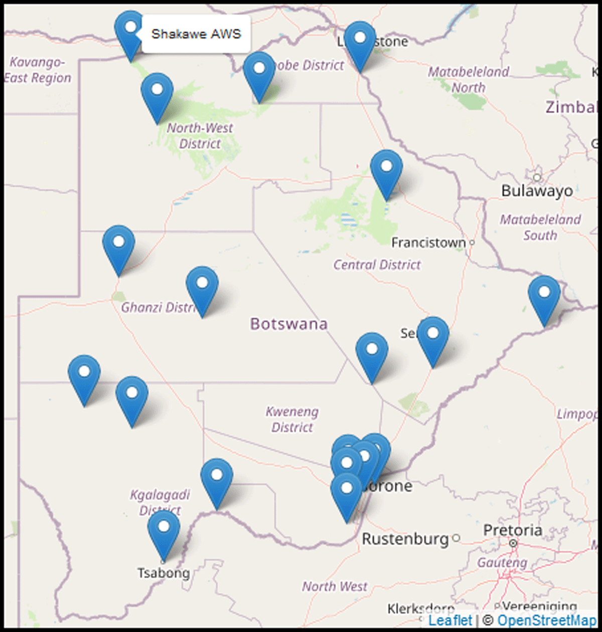
Figure 4
Visualising Botswana AWS using Algorithm 1.
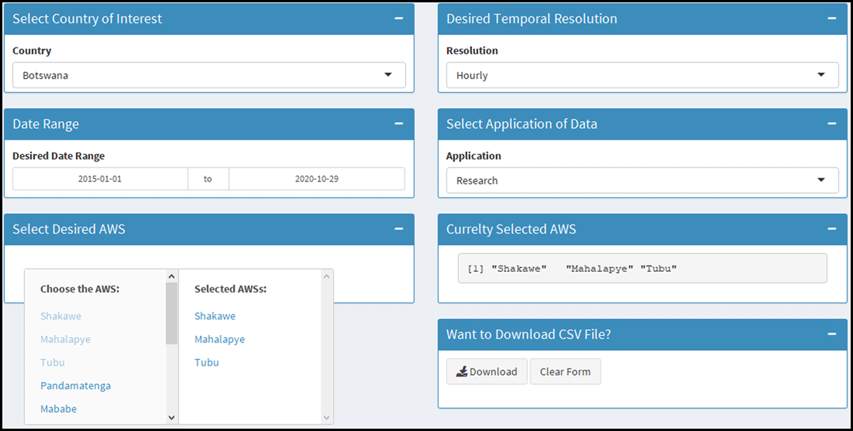
Figure 5
Screenshot of the SASSCAL WebSAPI for capturing user input when requesting weather data. The GUI allows end users to select the geographical location of interest (i.e., Botswana), temporal resolution, the AWS of interest and the downloading of data. The functionality of multi-input selection of AWSs provides end users with a feedback mechanisms to notify about the selected AWS as seen on the tab titled “Currently Selected AWS.” This is quite useful for a quick exploration of geographic locations before downloading data.
Algorithm 4
Dashboard design for dissemination.
| Input: It requires Algorithm 4. | ||
| Result: SASSCAL WebSAPI GUI | ||
| 1 | While (Interactive) do | |
| 2 | gui ← fluidPage (F ← DataScraper()) | |
| 3 | T← dashboardHeader(…), | |
| 4 | SDB← dashboardSidebar(…), | |
| 5 | B←dashboardBody(fluidRow(…))); | |
| 6 | server ← function(I,O) { Communicator(F) }; | |
| 7 | shinyApp(gui, server); | |
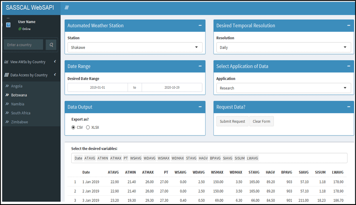
Figure 6
Screenshot of the SASSCAL WebSAPI’s GUI for data request, visualisation and extraction of data. In addition to selecting the desired AWS, temporal resolution, and the date range, the SASSCAL WebSAPI’s GUI allows end users to select the desired variables.
