
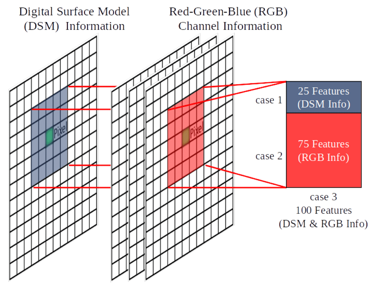
Figure 1
Feature extraction for SVM classification using a 5 × 5 neighborhood and a 1 channel (DSM only), 3 channel (RGB-only), or 4 channel (DSM & RGB) representation.
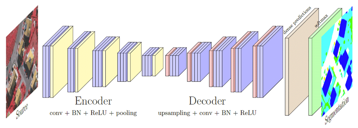
Figure 2
SegNet architecture from (Audebert, Le Saux, and Lefèvre, 2018; Badrinarayanan, Kendall, and Cipolla, 2017) utilizing a deep encoder-decoder structure for image segmentation and object classification. To perform nonlinear up-sampling, the SegNet decoder leverages pooling indices computed in the encoder layers of the network and connected from the encoder to the decoder via skip connections (Badrinarayanan, Kendall, and Cipolla, 2017).
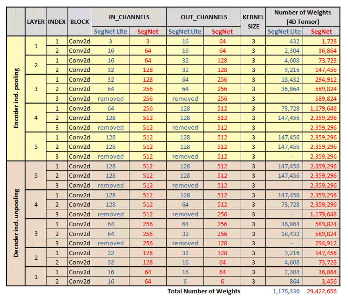
Figure 3
Comparison of Segnet and Segnet Lite architectures by number of indices per layer, number of input and output channels, weights per layer, and total weights. Note that the Segnet Lite architecture limits the number of layers per block to two and reduces the output channels for each layer by 75 percent.
Table 1
Comparative summary between our two Fully Convolutional Neural Network architectures, SegNet and SegNet Lite. These metrics are based off of Figure 3.
| NEURAL ARCHITECTURE | TOTAL PARAMETERS | CHANNELS (RELATIVE TO SEGNET) | KERNEL SIZE |
|---|---|---|---|
| SegNet | 29,422,656 | 1.0× | 3 |
| SegNet Lite | 1,176,336 | 0.25× | 3 |
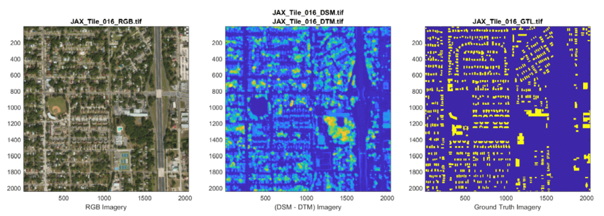
Figure 4
Sample tile from USSOCOM Urban 3D Challenge dataset for Jacksonville, FL showing RGB imagery (left), nDSM info (center), and annotated ground truth for building footprints (right).
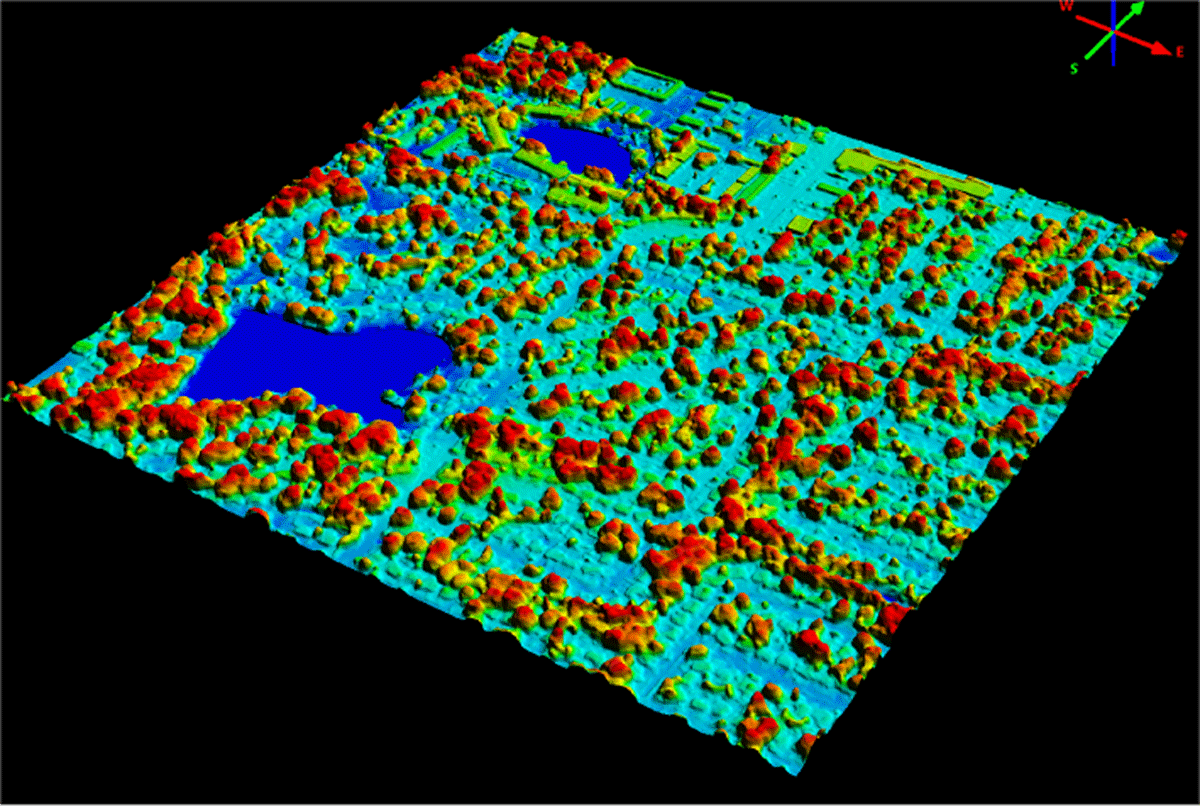
Figure 5
Another view of a sample nDSM (Jacksonville Tile 23) from the USSOCOM dataset.
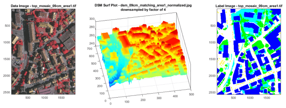
Figure 6
Sample tile from the ISPRS dataset for Vaihingen, Germany showing IRRG imagery (left), nDSM information (center), and color-coded ground truth for six object classes of interest (right).
Table 2
USSOCOM training and testing (in-sample and out-of-sample) procedures for SVM and SegNet. For evaluating the SegNet classifier on the USSOCOM dataset, we only test out-of-sample performance.
| CLASSIFIER ARCHITECTURE | |||
|---|---|---|---|
| TYPE OF DATASET | SVM | SEGNET | |
| Training | Jacksonville, FL | Tampa, FL | Tampa, FL |
| In-Sample Testing | Jacksonville, FL | – | – |
| Out-of-Sample Testing | Tampa, FL | Richmond, VA | Jacksonville, FL |
Table 3
ISPRS training and testing (in-sample and out-of-sample) procedures for our classification architectures: SVM, SegNet Lite, and SegNet.
| CLASSIFIER ARCHITECTURE | |||
|---|---|---|---|
| TYPE OF DATASET | SVM | SEGNET LITE | SEGNET |
| Training | Vaihingen tiles 1–12 | Vaihingen tiles 1–12 | Vaihingen tiles 1–12 |
| In-Sample Testing | Vaihingen tiles 13–16 | Vaihingen tiles 13–16 | Vaihingen tiles 13–16 |
| Out-of-Sample Testing | Potsdam* | Potsdam* | Potsdam* |
Table 4
SegNet – Classification performance by object type (accuracy only) for ISPRS in-sample (Vaihingen) and out-of-sample (Potsdam) validation using three training cases.
| OBJECTS OF INTEREST | SEGNET (ISPRS) | |||||
|---|---|---|---|---|---|---|
| VAIHINGEN | POTSDAM (9 CM) | |||||
| NDSM | IRRG | NDSM & IRRG | NDSM | IRRG | NDSM & IRRG | |
| Impervious surfaces | 0.8727 | 0.9520 | 0.9531 | 0.7127 | 0.7502 | 0.8374 |
| Buildings | 0.9549 | 0.9738 | 0.9722 | 0.6828 | 0.4571 | 0.7886 |
| Low vegetation | 0.8486 | 0.9299 | 0.9243 | 0.7320 | 0.7829 | 0.8589 |
| Trees | 0.9159 | 0.9488 | 0.9473 | 0.8846 | 0.8568 | 0.8643 |
| Cars | 0.9922 | 0.9969 | 0.9959 | 0.9865 | 0.9879 | 0.9912 |
| Clutter | 0.9995 | 0.9993 | 0.9996 | 0.9518 | 0.9598 | 0.9522 |
| Total | 0.7919 | 0.9003 | 0.8962 | 0.4752 | 0.3974 | 0.6463 |
Table 5
SegNet Lite – Classification performance by object (accuracy only) for ISPRS in-sample (Vaihingen) and out-of-sample (Potsdam) validation using three training cases.
| OBJECTS OF INTEREST | SEGNET LITE (ISPRS) | |||||
|---|---|---|---|---|---|---|
| VAIHINGEN | POTSDAM (9 CM) | |||||
| NDSM | IRRG | NDSM & IRRG | NDSM | IRRG | nDSM & IRRG | |
| Impervious surfaces | 0.8706 | 0.9519 | 0.9559 | 0.7123 | 0.7950 | 0.7827 |
| Buildings | 0.9539 | 0.9726 | 0.9735 | 0.8559 | 0.5554 | 0.6016 |
| Low vegetation | 0.8417 | 0.9322 | 0.9276 | 0.6077 | 0.7651 | 0.8182 |
| Trees | 0.9162 | 0.9490 | 0.9486 | 0.8687 | 0.8384 | 0.8669 |
| Cars | 0.9922 | 0.9969 | 0.9959 | 0.9864 | 0.9887 | 0.9871 |
| Clutter | 0.9992 | 0.9992 | 0.9996 | 0.9522 | 0.9551 | 0.9495 |
| Total | 0.7869 | 0.9009 | 0.9006 | 0.4916 | 0.4488 | 0.5030 |
Table 6
SVM – Classification performance by object (accuracy only) for in-sample (Vaihingen) and out-of-sample (Potsdam) validation using three training cases.
| OBJECTS OF INTEREST | 5 × 5 SVM CLASSIFIER (ISPRS) | |||||
|---|---|---|---|---|---|---|
| VAIHINGEN | POTSDAM (9 CM) | |||||
| NDSM | IRRG | NDSM & IRRG | NDSM | IRRG | NDSM & IRRG | |
| Impervious surfaces | 0.7812 | 0.8733 | 0.9320 | 0.6847 | 0.7665 | 0.8352 |
| Buildings | 0.7931 | 0.8914 | 0.9567 | 0.7550 | 0.5257 | 0.6913 |
| Low vegetation | 0.8309 | 0.8715 | 0.8978 | 0.7246 | 0.7768 | 0.8147 |
| Trees | 0.7537 | 0.9101 | 0.9317 | 0.7464 | 0.8325 | 0.8214 |
| Cars | 0.9688 | 0.9915 | 0.9928 | 0.8530 | 0.9862 | 0.9832 |
| Clutter | 0.9922 | 0.9997 | 0.9997 | 0.9412 | 0.9436 | 0.9429 |
| Total | 0.5600 | 0.7687 | 0.8553 | 0.3266 | 0.4157 | 0.5444 |
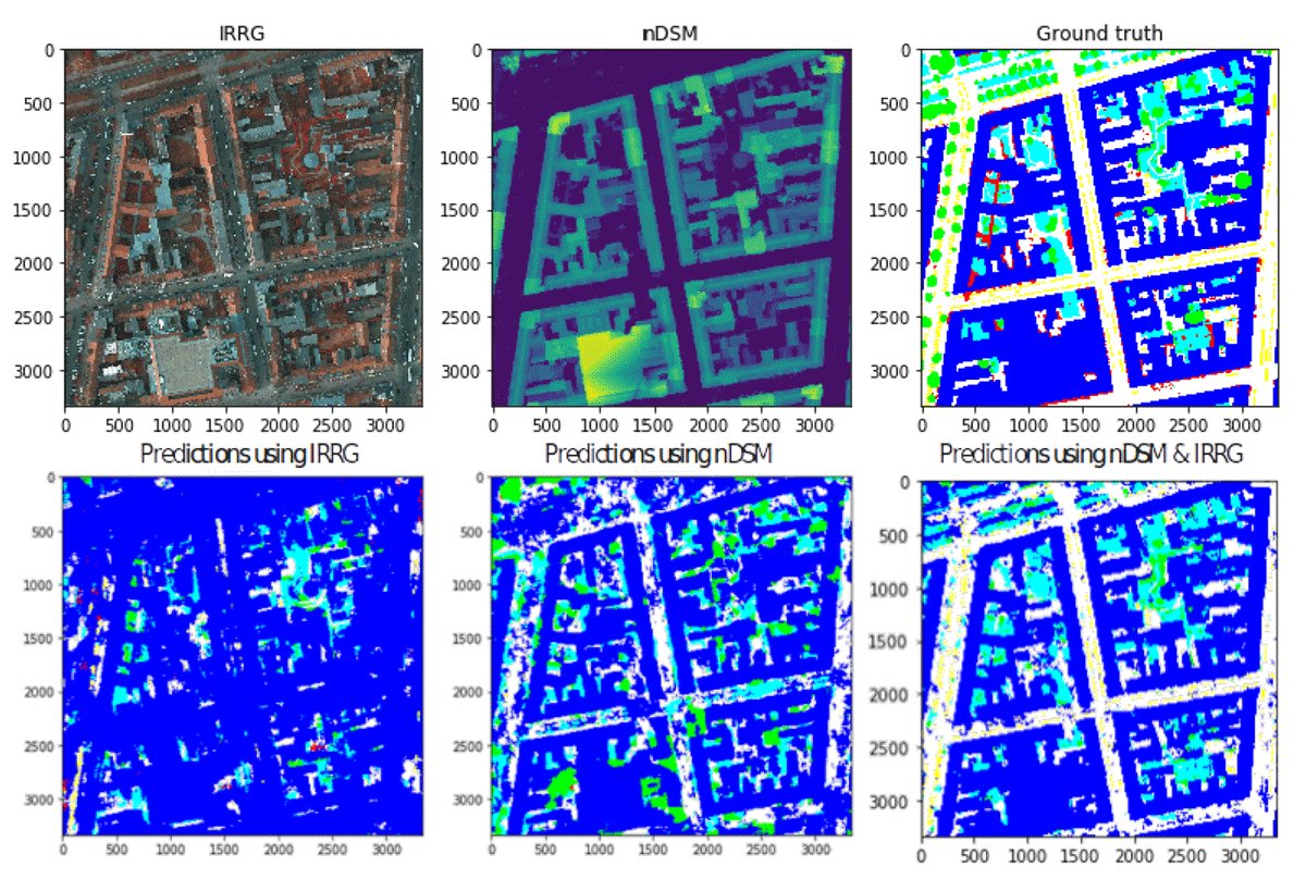
Figure 7
Qualitative out-of-sample classification performance for SegNet classifier applied to ISPRS Potsdam data. From left to right, the top row shows IRRG imagery, nDSM information, color-coded ground truth annotations. From left to right, bottom row display predictions when trained with (i) IRRG info only, (ii) nDSM info only, and (iii) combined IIRG & nDSM info.
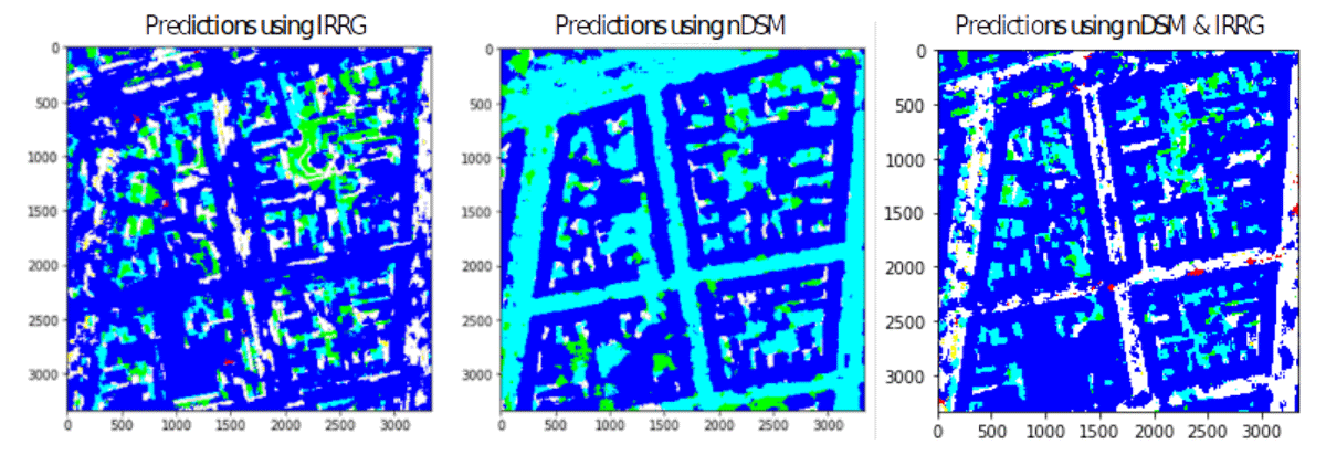
Figure 8
Qualitative out-of-sample classification performance for SegNet Lite classifier for the same tile as used in Figure 7 from the ISPRS Potsdam data, display predictions when trained with (i) IRRG info only, (ii) nDSM info only, and (iii) combined IIRG & nDSM info.
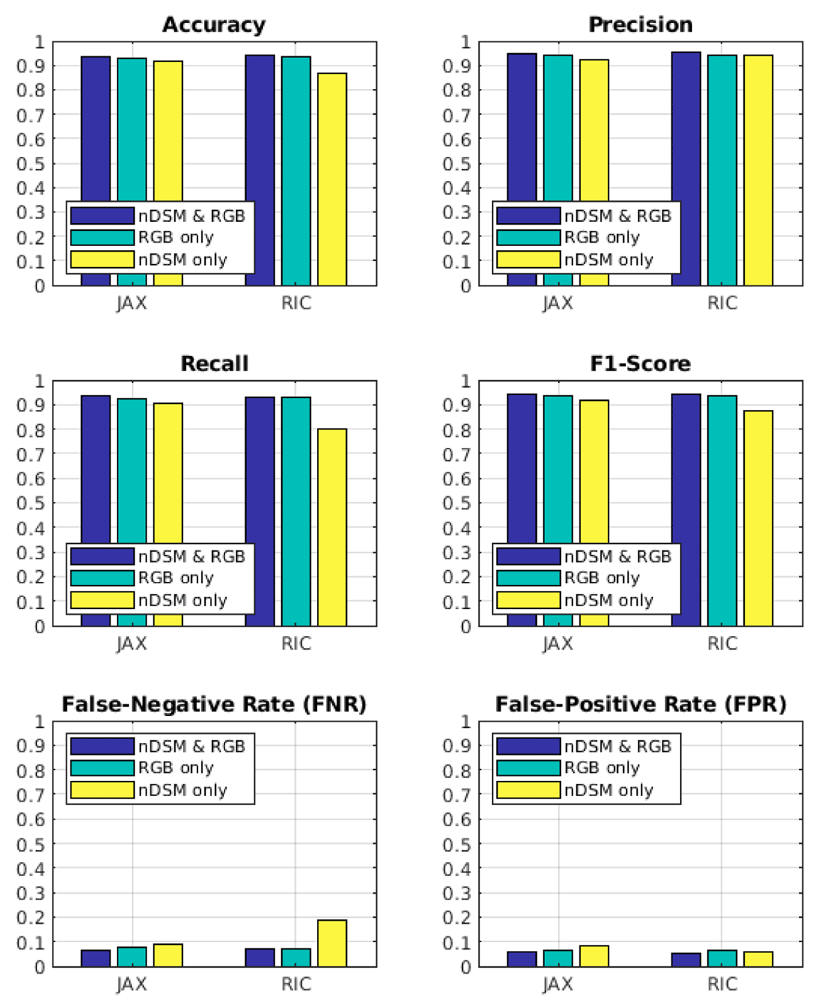
Figure 9
Cross-city building classification performance for the USSOCOM dataset using SegNet classifiers. Classifiers are color-coded: nDSM & RGB in blue, RGB-only in green, and nDSM-only in yellow. Note that JAX corresponds to out-of-sample testing with tiles from Jacksonville, and RIC corresponds to out-of-sample testing with tiles from Richmond.
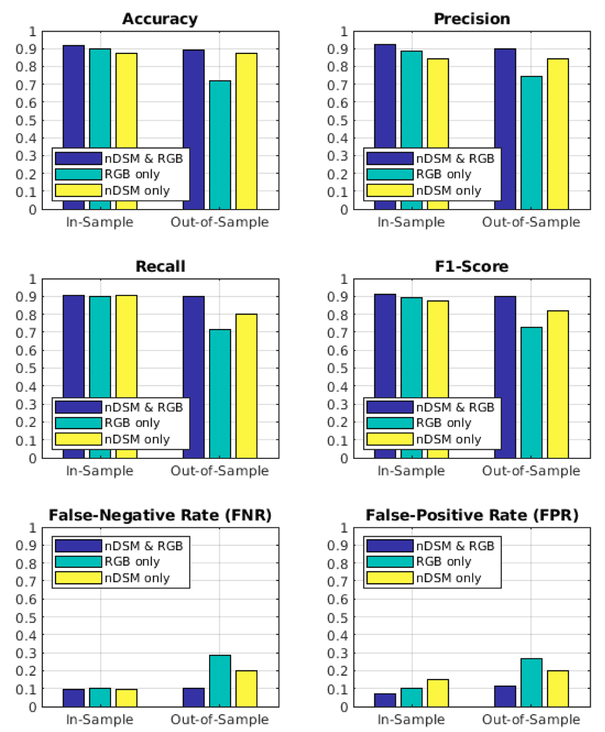
Figure 10
In-sample and out-of-sample building classification performance for the USSOCOM dataset using SVM classifiers. Classifiers are color-coded: nDSM & RGB in blue, RGB-only in green, and nDSM-only in yellow.
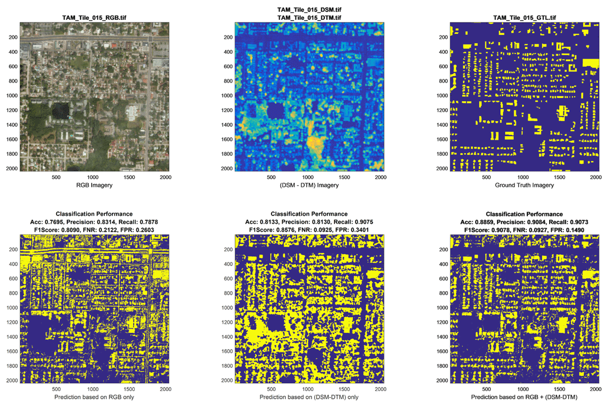
Figure 11
Qualitative out-of-sample classification performance for SVM classifiers applied to USSOCOM data. From left to right, the upper row shows RGB imagery, nDSM (DSM-DTM) information, and ground truth, i.e. annotated building footprints, for Tampa tile #014. From left to right, the lower row shows predicted building footprints when training on (i) nDSM information only, (ii) RGB imagery only, and (iii) combined RGB & nDSM information.
Table 7
SegNet – Balanced building classification performance metrics for cross-city (out-of-sample) validation following procedures 1 and 2 in table 2. In procedure 1 (left three columns), SegNet was trained on tiles from Tampa, Florida, and tested on tiles from Jacksonville, Florida. In procedure 2 (right three columns), SegNet was trained on tiles from Tampa, Florida, and tested on tiles from Richmond, Virginia.
| CLASSIFICATION METRICS | SEGNET (US SOCOM) | |||||
|---|---|---|---|---|---|---|
| TRAIN TAM TEST JAX | TRAIN TAM TEST RIC | |||||
| NDSM | RGB | NDSM & RGB | NDSM | RGB | NDSM & RGB | |
| Accuracy | 0.9164 | 0.9298 | 0.9367 | 0.8690 | 0.9339 | 0.9386 |
| Precision | 0.9245 | 0.9412 | 0.9451 | 0.9425 | 0.9416 | 0.9512 |
| Recall | 0.9105 | 0.9245 | 0.9341 | 0.8122 | 0.9307 | 0.9298 |
| F1 Score | 0.9175 | 0.9328 | 0.9396 | 0.8725 | 0.9361 | 0.9404 |
| False Negative Rate | 0.0895 | 0.0755 | 0.0659 | 0.1878 | 0.0693 | 0.0702 |
| False Positive Rate | 0.0829 | 0.0643 | 0.0604 | 0.0610 | 0.0626 | 0.0518 |
Table 8
SVM – Balanced building classification performance metrics for in-sample and out-of-sample testing on the USSOCOM dataset.
| CLASSIFICATION METRICS | 5 × 5 SVM CLASSIFIER (USSOCOM) | |||||
|---|---|---|---|---|---|---|
| IN-SAMPLE TESTING | OUT-OF-SAMPLE TESTING | |||||
| NDSM | RGB | NDSM & RGB | NDSM | RGB | NDSM & RGB | |
| Accuracy | 0.8763 | 0.8978 | 0.9178 | 0.8763 | 0.7212 | 0.8931 |
| Precision | 0.8438 | 0.8850 | 0.9214 | 0.8438 | 0.7467 | 0.9003 |
| Recall | 0.9047 | 0.8996 | 0.9023 | 0.8000 | 0.7126 | 0.8963 |
| F1 Score | 0.8732 | 0.8922 | 0.9117 | 0.8200 | 0.7292 | 0.8983 |
| False Negative Rate | 0.0953 | 0.1004 | 0.0977 | 0.2000 | 0.2874 | 0.1037 |
| False Positive Rate | 0.1488 | 0.1039 | 0.0684 | 0.2000 | 0.2693 | 0.1105 |
Table 9
Average training times (in seconds) for SVM classifiers when using smaller sample proportions for training on USSOCOM data.
| SAMPLE PROPORTION FOR TRAINING | 0.0001% | 0.001% | 0.01% | 0.1% |
|---|---|---|---|---|
| SVM Training Times (sec) | 0.1 | 1.5 | 180 | 24,000 |
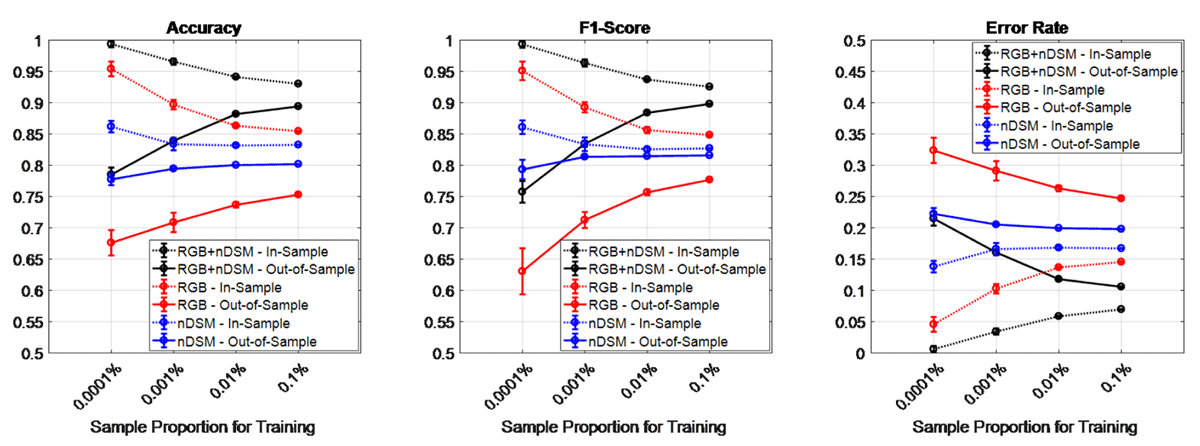
Figure 12
Impact of sample proportion on in-sample (dotted lines) and out-of-sample (solid lines) SVM classification performance on the USSOCOM Jacksonville, FL dataset. The study compares three input data scenarios, (a) RGB & nDSM (black), (b) RGB-only (red), and (c) nDSM-only (blue). From left to right, the individual plots show accuracy, F1-score, and error rate as a function of sample proportion.
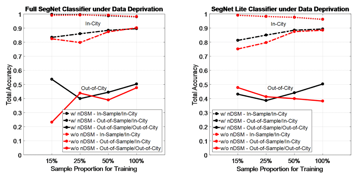
Figure 13
Impact of sample proportion on classification performance using SegNet (left) and SegNet Lite (right) on ISPRS data.