
Table 1
Steps of the six methodologies.
| GrHyMM | UMLDW | MDBE | PDM | GRAnD | GQM | VMQD* | |
|---|---|---|---|---|---|---|---|
| Requirement Analysis | goals, tasks | goals, tasks | queries in SQL | queries in SQL | goals, decisions | goals, questions, metrics | visualized questions, metrics, dimensionality |
| Minimal Granularity | minimally detailed metrics | ||||||
| Ideal Schema | ideal facts, ideal dimensions | ideal facts, ideal dimensions | |||||
| Source Analysis | independent, source system schema | independent, CWM | independent | independent | independent | independent, potential schema | potential transactions, attributes, partly dependent, |
| Integration | potential schema vs.ideal schema | potential schema vs.ideal schema | |||||
| Reconciliation | DB integrity | consistent UML multidimensional schema | DB integrity | ||||
| Multidimensional Modeling | facts, attribute tree for facts, remodeling | cubes, dimensions, hierarchies, measures | dimensions and facts from tables | Date dimension and Attribute dimensions for factsMeER | Derived from requirement analysis schemas | MeER | |
| Schema Selection | MeER related to questions | ||||||
| Manual Refinement | modified automatically generated schema | ||||||
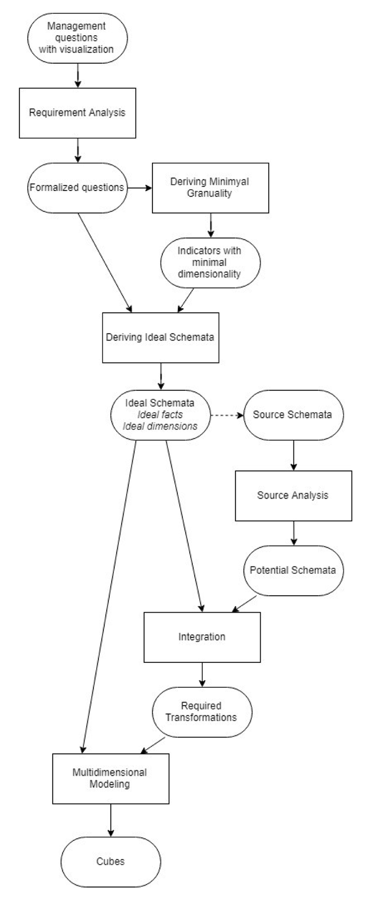
Figure 1
Framework of VMQD.
Table 2
Management question analysis.
| Indicator | the indicator I to be produced with u unit(s) in the upper right index and af aggregate function(s) in the bottom right index, | |
| unit(s) | ||
| aggregate function(s) | ||
| visualization | the v visualization with the type vt (table, line diagram, bar graph, etc. …) and optional s slicers (values can be D{a} dimensional attribute, D{v} subset of concrete values, or a D{a} dimensional attribute in the d detail of another I indicator on the same dashboard) | |
| slicer(s) | ||
| detail(s) | d details with D{a} dimensional attribue(s), with optional aggregation. d values e.g.: row, column, category, y indicator |
Table 3
Optimizations’ notations.
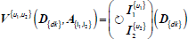
| Combining indicators I1 and I2 with the same dimensionality. We create the Descartes multiplier of the two indicators. | |
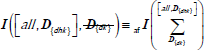 | The value of the indicator I can be obtained by summing through dimension D (roll up) with the aggregate function in the lower left index of I. Calculating the aggregation from D{dk} at the bottom of the Summa symbol to the level at the top of the Summa sign (all or D{dhk} hierarchy level, leaving the original key. This is referred to as  . . |
| A and B are dimensions of indicators I1 and I2 and I1 is proper subset of I2. |
Table 4
Data loadings’ transformation notations.
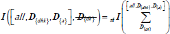 | The value of the indicator I can be obtained by summing through D dimension (roll up) with the aggregate function in the lower left index of I. This is an aggregation is from D{dk} at the bottom of the Summa symbol to the level at the top of the Summa Sign (all or D{dhk} hierarchy level, leaving the original key. This is referred to as . |
| Deduplicate the values of D dimensions’ D{dk}. key. Summarize the indicator with the af aggregate function in the lower left index, while leaving the first element of attribute values. | |
| Expand the dimensionality of indicator I. The Descartes multiplier of the original indicator with the dimension to be expanded. | |
 | Pivoting I indicator values through D{a} dimensional attribute. We create several new indicators corresponding to the occurrence values of the attribute. |
| Combining I1 I2 indicators with the same dimensionality. We create the Descartes multiplier of the two indicators. | |
 | Unpivoting I1 I2 indicators with the same dimensionality into V indicator values and A attribute set with the indicators’ name |
| The sum of pivoted indicator values along the occurrence values of D{a} attribute. |
Table 5
Question1 analysis.
| Indicator | how many days completed (activity) | Activity{day} | |
| unit(s) | day | ||
| aggregate function(s) | how many (sum) | ||
| visualization | table | ||
| slicer(s) | March | ||
| detail(s) | student | ||
| daily step category |
[i]
Table 6
Question2 analysis.
| Indicator | averagely completed days | ||
| unit(s) | day | ||
| aggregate function(s) | average | ||
| visualization | table | ||
| slicer(s) | March | ||
| detail(s) | gender | ||
| daily step category |
[i]
Table 7
Question3 analysis.
| Indicator | Daily steps | ||
| unit(s) | steps | ||
| aggregate function(s) | average | ||
| visualization | radar chart | ||
| slicer(s) | March | ||
| detail(s) | day of the week | ||
| men, women, all |
[i]
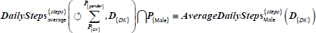
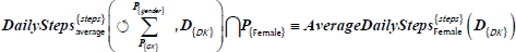
Table 8
10-minute normalized steps’ property mapping.
| OLTP system (extract) | transform | OLAP system (load) |
|---|---|---|
| S{10mNS} | => | 10minNS{step} |
| S{DK} | => | D{DK} |
| S{TK} | => | T{TK} |
| S{PK} | => | P{TK} |
[i]
Table 9
Person dimension’s property mapping.
| OLTP system (extract) | transform | OLAP system (load) |
|---|---|---|
| P{PK} | => | P{PK} |
| P{GenderEn} | => | P{gender} |
[i]
Table 10
Date dimension’s property mapping.
| OLTP system (extract) | transform | OLAP system (load) |
|---|---|---|
| D{DK} | => | D{DK} |
| left(D{DK}, 6) | D{MK} | |
| D{DOW} | D{DoW}&“–”&D{weekdayEn} | D{weekday} |
| D{weekdayEn} |
[i]
Table 11
Month dimension-hierarchy’s property mapping.
| OLTP system (extract) | transform | OLAP system (load) |
|---|---|---|
| D{DK} | left(D{DK}, 6) | DM{MK} |
| D{monthStrEn} | => | DM{month} |
[i]
Table 12
Walk intensity dimension’s property mapping.
| OLTP system (extract) | transform | OLAP system (load) |
|---|---|---|
| I{IK} | => | I{IK} |
| I{IK} | I{IK}&“–”& D{sscEn} | I{dsc} |
| D{sscEn} |
[i]

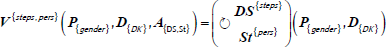
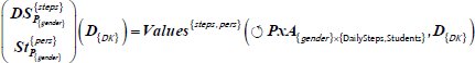
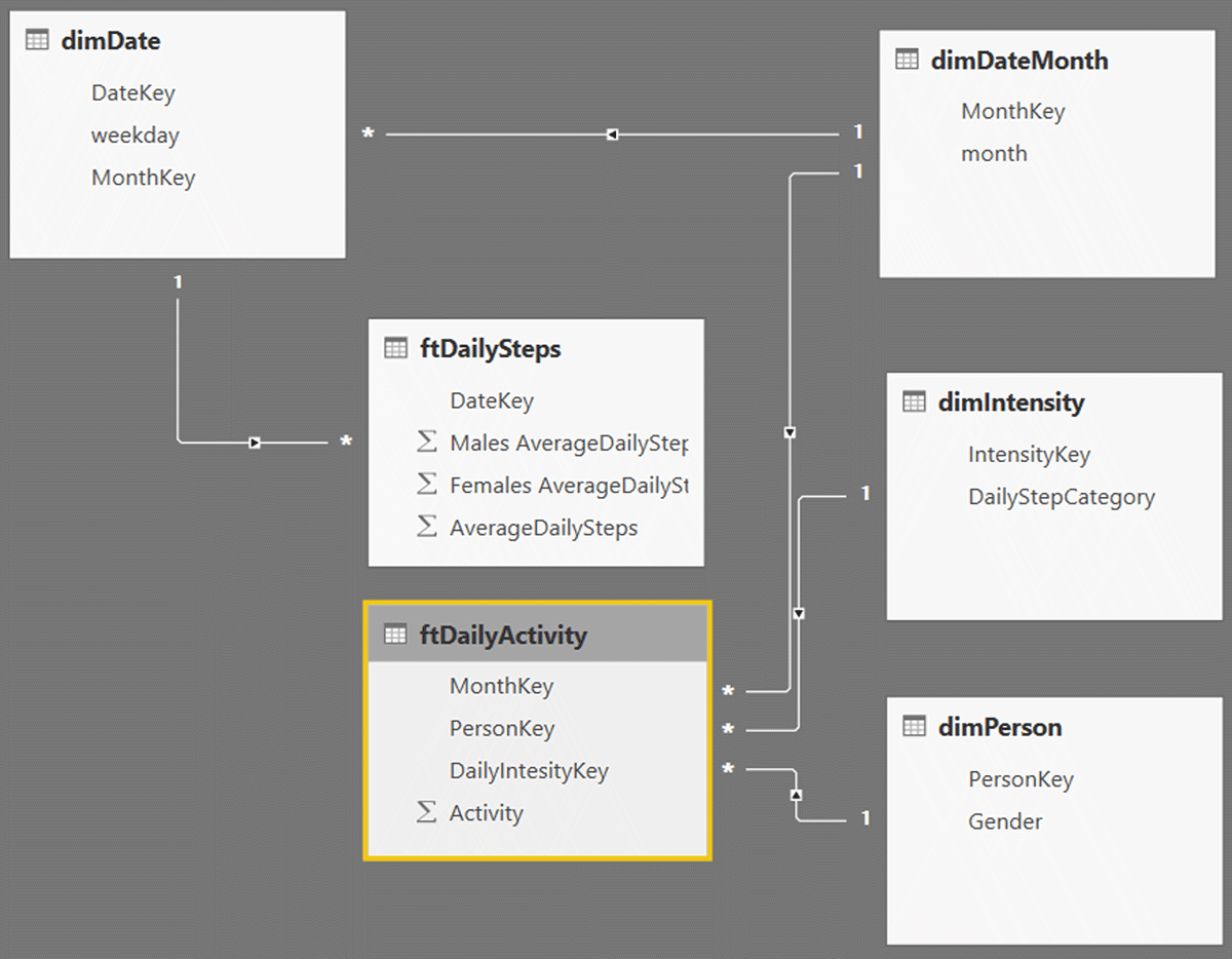
Figure 2
Galaxy schema of the optimal cube.
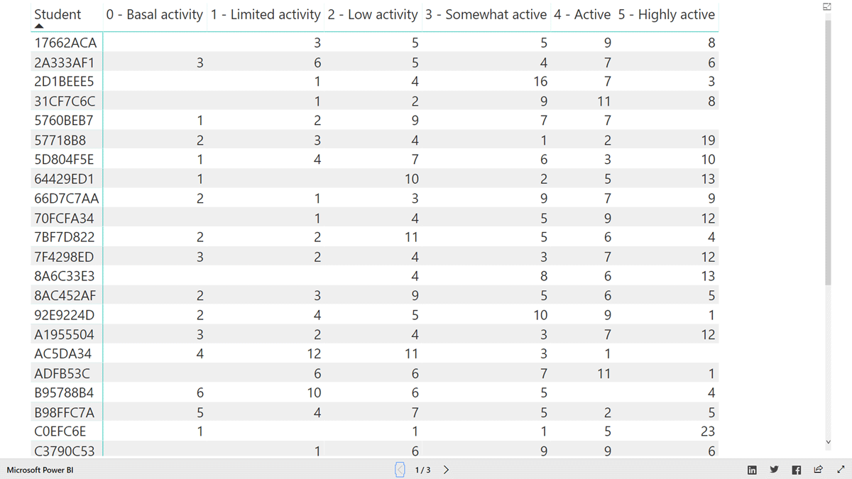
Figure 3
Table visualization of question1.
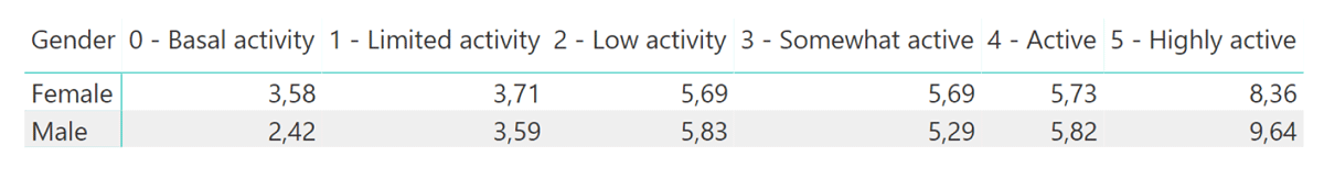
Figure 4
Table visualization of question2.
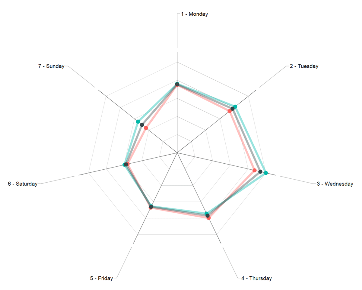
Figure 5
Radar chart visualization of question3.