
Table 1
The 20 Data Bottles and their descriptions extracted from a Data Lake created for this particular case study.
| Bottles | Descriptions |
|---|---|
| ID | ID about claims, policy, person, etc. |
| CUSTOMER | Policyholder’s attributes embodied in insurance policies: name, sex, age, address, etc. |
| CUSTOMER_PROPERTY | Customer related with the property data. |
| DATES | Dates of about claims, policy, visits, etc. |
| GUARANTEES | Coverage and guarantees of the subscribed policy. |
| ASSISTANCE | Call center claim assistance. |
| PROPERTY | Data related to the insured object. |
| PAYMENTS | Policy payments made by the insured. |
| POLICY | Policy contract data, including changes, duration, etc. |
| LOSS ADJUSTER | Information about the process of the investigation but also about the loss adjuster. |
| CLAIM | Brief, partial information about the claim, including date and location. |
| INTERMEDIARY | Information about the policies’ intermediaries. |
| CUSTOMER_OBJECT_RESERVE | The coverage and guarantees involved in the claim. |
| HISTORICAL_CLAIM | Historical movements associated with the reference claim. |
| HISTORICAL_POLICY | Historical movements associated with the reference policy (the policy involved in the claim). |
| HISTORICAL_OTHER_POLICIES | Historical movements of any other policy (property or otherwise) related to the reference policy. |
| HISTORICAL_OTHER_CLAIM | Historical claim associated with the reference policy (excluding the claim analyzed). |
| HISTORICAL_OTHER_POL_CLAIM | Other claim associated with other policies not in the reference policy (but related to the customer). |
| BLACK_LIST | Every participant involved in a fraudulent claim (insured, loss-adjuster, intermediary, other professionals, etc.) |
| CROSS VARIABLES | Several variables constructed with the interaction between the bottles. |
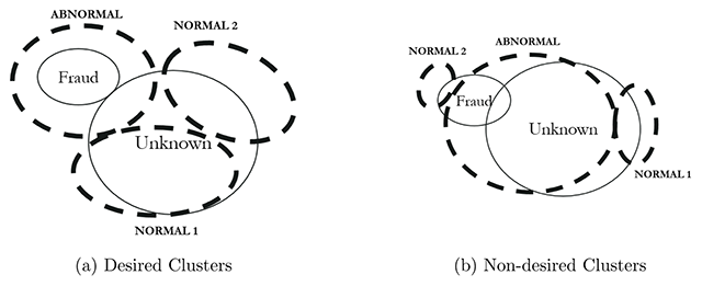
Figure 1
Possible clusters. (a) shows a separable and compact cluster of the abnormal points. On the other side, (b) shows abnormal and normal cases uniformly distributed.
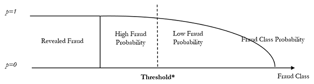
Figure 2
Schematic representation of the desired threshold which is expected to split high fraud probability cases from low fraud probability cases.
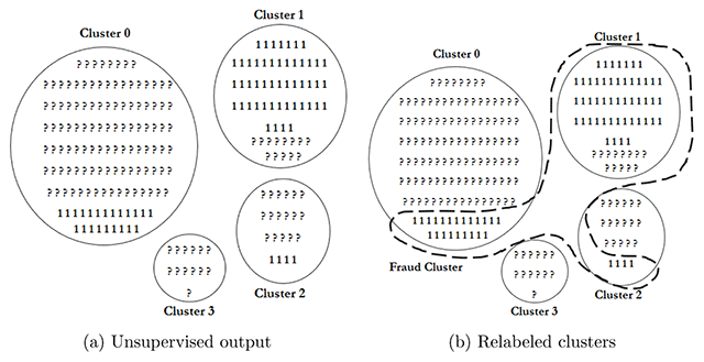
Figure 3
Cluster Example Output. (a) shows an example of a cluster algorithm output over a sample of data points. (b) shows how the Cluster Score choose the points that are relabeled as fraud cases (points inside the doted line).
Algorithm 1
Unsupervised algorithm
| Data: Load transformed data-set. Oversample the fraud cases in order to have the same amount as the number of unknown cases. | |
| 1 | for k ∈ K = {model1, model2, …} where K is a set of unsupervised models. do |
| 2 | for i ∈ I where I is a matrix of parameter vectors containing all possible combinations of the parameters in model k do |
| 3 | We fit the model k with the parameters i to the oversampled data-set. |
| 4 | We get the J clusters: {C1, C2, …, CJ} for the combination {k, i}, i.e., |
| 5 | For Ck,i we calculate C1 Score and C2 Score and we obtain the cluster score CSk,i, based on the acceptance threshold t*. |
| 6 | Save the cluster score result CSk,i ∈ CSK,I, where CSK,I is the cluster score vector for each pair {k, i}. |
| 7 | end |
| 8 | end |
| 9 | Choose the optimal CS* where CS* = max{CSK,I} |
| 10 | Relabel the fraud variable using the optimal clustering model derived from CS*. Each unknown case in a fraud cluster is now equal to 1, known fraud cases are equal to 1 and remaining cases are equal to 0. |
Algorithm 2
Supervised algorithm.
| Data: Load relabeled data-set. | |
| 1 | for modeli ∈ M′ = {M, S} where M is the set of supervised individual models M and S the set of stacking models from M do |
| 2 | for {traink, testk} folds in the Stratified k-Folds do |
| 3 | We apply PCA to folder traink and save the weights/parameters. |
| 4 | if Oversample==True then train′k = oversample (traink) where oversampling is applied to 50/50 using the ADASYN method. |
| 5 | else train′k = train′k and the balanced subsampling option is activated. |
| 6 | Fit the modeli in train′k, where modeli ∈ M′ = {M, S}. |
| 7 | Transform testk with PCA’s weights/parameters and get predicted probabilities pk of testk using modeli. |
| 8 | Save the probabilities pk in Pi, where Pi is the concatenation of modeli’s probabilities. |
| 9 | end |
| 10 | for ∀ti ∈ [0, 1], where t is a probability threshold of the modeli to consider a case as fraudulent do |
| 11 | if Pi ≥ ti then Pi = 1 |
| 12 | else Pi = 0 |
| 13 | Using Pi, where now Pi is a binary list, we calculate, with β = 2. |
| 14 | Save FScorei,t in FScorei, a list of vectors of modeli with FScore results for each t. |
| 15 | end |
| 16 | We get FScorei* = max{FScorei(t)}. |
| 17 | end |
Table 2
Unsupervised model results.
| Model | n Clusters | C1 | C2 | CS (α = 2) |
|---|---|---|---|---|
| Mini-Batch K-Means | 4 | 96.6% | 96.6% | 96.6% |
| Isolation Forest | 2 | 51.5% | 51.1% | 51.4% |
| DBSCAN | 2 | 50.2% | 49.8% | 50.1% |
| Gaussian Mixture | 5 | 95.0% | 95.0% | 96.3% |
| Bayesian Mixture | 6 | 96.5% | 96.4% | 96.5% |
Table 3
Oversampled Unsupervised Mini-Batch K-Means.
| Clusters | Fraud | Percentage |
|---|---|---|
| 0 | 0 | 2% |
| 0 | 1 | 98% |
| 1 | 0 | 99% |
| 1 | 1 | 1% |
| 2 | 0 | 100% |
| 2 | 1 | 0% |
| 3 | 0 | 1% |
| 3 | 1 | 99% |
Table 4
Supervised model results.
| Model | Cluster Recall | Original Recall | Precision | F-Score |
|---|---|---|---|---|
| ERT-ss | 0.9734 | 0.9840 | 0.6718 | 0.8932 |
| ERT-os | 0.9647 | 0.9819 | 0.6937 | 0.8948 |
| GB | 0.9092 | 0.9376 | 0.6350 | 0.8369 |
| LXGB | 0.8901 | 0.9249 | 0.7484 | 0.8576 |
| Stacked-ERT | 0.8901 | 0.9283 | 0.7524 | 0.8587 |
| Stacked-GB | 0.8947 | 0.9287 | 0.7630 | 0.8649 |
| Stacked-LXGB | 0.9180 | 0.9464 | 0.6825 | 0.8588 |
Table 5
Model Robustness Check.
| Original Value | Prediction | Cases |
|---|---|---|
| Non-Investigated | Non-Fraud | 29.631 |
| Fraud | Non-Fraud | 0 |
| Non-Investigated | Fraud | 415 |
| Fraud | Fraud | 271 |
| (a) ERT-ss Robustness Check | ||
| Original Value | Prediction | Cases |
| Non-Investigated | Non-Fraud | 29.656 |
| Fraud | Non-Fraud | 8 |
| Non-Investigated | Fraud | 390 |
| Fraud | Fraud | 263 |
| (b) ERT-os Robustness Check | ||
Table 6
Base Model Final Results.
| Original Value | Prediction | Cases |
|---|---|---|
| Non-Investigated | Non-Fraud | 29.631 |
| Fraud | Non-Fraud | 0 |
| Non-Fraud | Fraud | (415 – 333) = 82 |
| Fraud | Fraud | (271 + 333) = 604 |
Table 7
Oversampled Unsupervised Mini-Batch K-Means.
| Clusters | Fraud | Percentage |
|---|---|---|
| 0 | 0 | 99.4% |
| 0 | 1 | 0.6% |
| 1 | 0 | 0.7% |
| 1 | 1 | 99.3% |
| 2 | 0 | 2.6% |
| 2 | 1 | 97.4% |
Table 8
Base Model with the machine-learning process applied.
| Period | Jan 15–Jan 17 | Jan 15–Jan 18 |
|---|---|---|
| Claims | 303,166 | 519,921 |
| Observed Fraud | 2,641 | 4,623 |
| Cluster Score | 96.59% | 96.89% |
| Recall Score ERT-ss | 97.34% | 96.31% |
| Precision Score ERT-ss | 67.18% | 89.35% |
| F-Score ERT-ss | 89.32% | 94.84% |
| Recall Score ERT-os | 96.47% | 96.44% |
| Precision Score ERT-os | 69.37% | 92.18% |
| F-Score ERT-os | 89.48% | 95.56% |