
Algorithm 1
The GeoSim Algorithm.
| Input: V: set of all nodes in the social network, E: set of all edges in the network, I: set of all interests for all nodes and K: number of communities. | |
| Output: C: set of detected communities. | |
| 1: | procedure GEOSIM(V, E, I, K) |
| 2: | C = createRandomClusters(V, K); |
| 3: | distances = apsp(V, E) // all-pairs shortest paths |
| 4: | while community_variation > threshold do |
| 5: | for c ∈ C do |
| 6: | max_degree = 0 |
| 7: | for node ∈ c do |
| 8: | if node.degree > max_degree then |
| 9: | mean_nodes[c] = node |
| 10: | max_degree = node.degree |
| 11: | end if |
| 12: | end for |
| 13: | end for |
| 14: | for v ∈ V do |
| 15: | min_gss = ∞ |
| 16: | for mean_node ∈ mean_nodes do |
| 17: | distances = distances(mean_node, v) |
| 18: | calculate gss using equation 1 |
| 19: | if gss < min_gss then |
| 20: | c_id = mean_node.community |
| 21: | min_gss = gss |
| 22: | end if |
| 23: | end for |
| 24: | C[c_id].addNode(v) |
| 25: | end for |
| 26: | end while |
| 27: | return C; |
| 28: | end procedure |
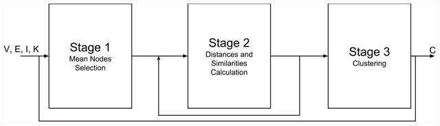
Figure 1
The three stages of the proposed GeoSim algorithm, where V is the set of all nodes in the social network, E is the set of all edges in the network, I is the set of all interests for all nodes and K is the number of communities.
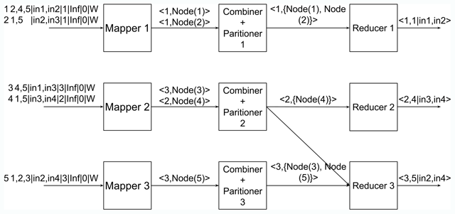
Figure 2
An example of the map and reduce phases of the Mean Nodes Selection stage of the GeoSimMR algorithm.
Algorithm 2
Mean Nodes Selection Stage.
| Input: input_file: The input file, a file containing the nodes information. | |
| Output: output_file: A file containing a set key-value pairs, the key is the community id and the value is the node id and its interests. | |
| 1: | procedure MAP(line) |
| 2: | node = parseNode(line) |
| 3: | node.calculateFriendsNumber() |
| 4: | emit(node.communityId, node) |
| 5: | end procedure |
| 6: | |
| 7: | procedure REDUCE(communityId, nodesList) |
| 8: | maxFriends = 0 |
| 9: | for node ∈ nodesList do |
| 10: | if node.friendsNumber > maxFriends then |
| 11: | meanNode = node |
| 12: | maxFriends = node.friendsNumber |
| 13: | end if |
| 14: | end for |
| 15: | emit(communityId, node.printIdAndInterests()) |
| 16: | end procedure |
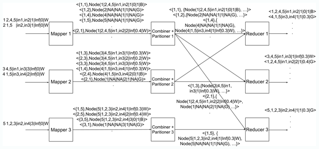
Figure 3
An example of the map and the reduce phases of the Distances and Similarities Calculation stage of the GeoSimMR algorithm.
Algorithm 3
Distances and Similarities Calculation Stage.
| Input: input_file: The input file which contains the nodes information., meanNodes: A list of mean nodes obtained from the Mean Nodes Selection stage. | |
| Output: output_file: A file containing the distances and the similarities from each node to all mean nodes. | |
| 1: | procedure MAP(line) |
| 2: | node = parseNode(line) |
| 3: | for meanNode ∈ meanNodes do |
| 4: | if isFirstIteration then |
| 5: | node.calculateSimilarity(meanNode) |
| 6: | end if |
| 7: | if node == meanNode||node.v == G then |
| 8: | if node == meanNode then |
| 9: | node.distance = 0 |
| 10: | end if |
| 11: | for friendinnode.friends do |
| 12: | friend.v = G |
| 13: | friend.distance = node.distance + 1 |
| 14: | emit({meanNode.communityId, |
| 15: | friend.id}, friend) |
| 16: | end for |
| 17: | end if |
| 18: | emit({meanNode.communityId, node.id}, node) |
| 19: | end for |
| 20: | end procedure |
| 21: | |
| 22: | procedure REDUCE(communityId, nodeId, nodesList) |
| 23: | outNode.communityId = nodeId |
| 24: | outNode.id = communityId |
| 25: | outNote.friends = getFriends(nodesList) |
| 26: | outNote.interests = getInterests(nodesList) |
| 27: | for node ∈ nodesList do |
| 28: | if outNode.distance > node.distance then |
| 29: | outNode.distance = node.distance |
| 30: | end if |
| 31: | if outNode.similarity < node.similarity then |
| 32: | outNode.similarity = node.similarity |
| 33: | end if |
| 34: | if outNode.v < node.v then |
| 35: | outNode.v = node.v |
| 36: | end if |
| 37: | end for |
| 38: | emit (outNode.id, outNode.printInfo()) |
| 39: | end procedure |
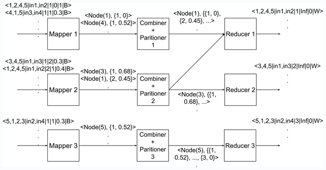
Figure 4
An example of the map and reduce phases of the Clustering stage of the GeoSimMR algorithm.
Algorithm 4
Clustering Stage.
| Input: input_file: The output file of the Distances and Similarities Calculation. | |
| Output: output_file: List of all nodes and their detected communities. | |
| 1: | procedure MAP(line) |
| 2: | node = parseNode(line) |
| 3: | Calculate GSS using equation 1 |
| 4: | emit(node, GSS) |
| 5: | end procedure |
| 6: | |
| 7: | procedure REDUCE(communityId, communityGSSPairs) |
| 8: | minScore = inf |
| 9: | for pair ∈ communityGSSPairs do |
| 10: | if pair.GSS < minScore then |
| 11: | minScore = pair.GSS |
| 12: | communityId = pair.communityId |
| 13: | end if |
| 14: | end for |
| 15: | node.communityId = communityId |
| 16: | emit(node.id, node.printInfo()) |
| 17: | end procedure |
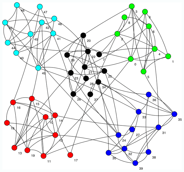
Figure 5
The detected communities in the network by the GeoSim algorithm (α = 0.7).
Table 1
DBLP authors used as a ground truth in the community detection experiment.
| Database | Data Mining | Artificial Intelligence |
|---|---|---|
| V. S. Subrahmanian | Alex Beutel | Donald Perlis |
| David j. DeWitt | Rakesh Agrawal | Mary Anne Williams |
| Michael Stonebraker | Ramakrishnan Srikant | Wei Liu |
| Hans Peter Kriegel | Christos Faloutsos | Keith Johnson |
| Timos K. Sellis | Flavio Figueiredo | Sanjay Chawla |
| Laura M. Haas | Bruno Ribeiro | James Bailey |
| H. V. Jagadish | Bussara M. Almeida | Christopher Leckie |
| Vassilis J. Tsotras | Yasuko Matsubara | Kotagiri Ramamohanarao |
| Raymond T. Ng | lei li | Daren Ler |
| Christian S. Jensen | Evangelos E. Papalexakis | Irena Koprinska |
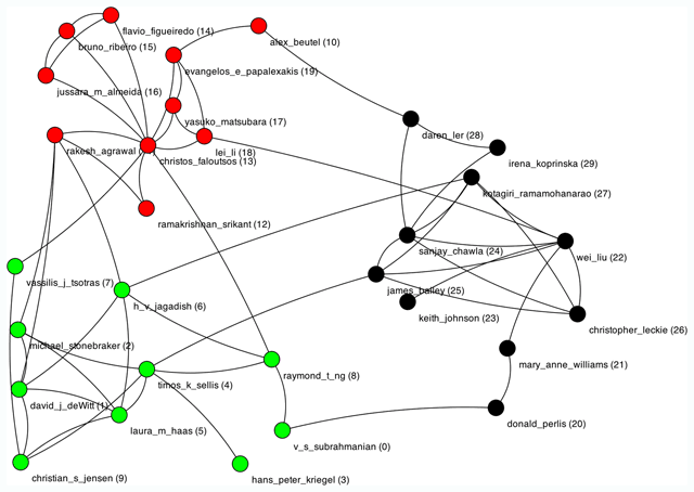
Figure 6
Detected communities in a DBLP graph.
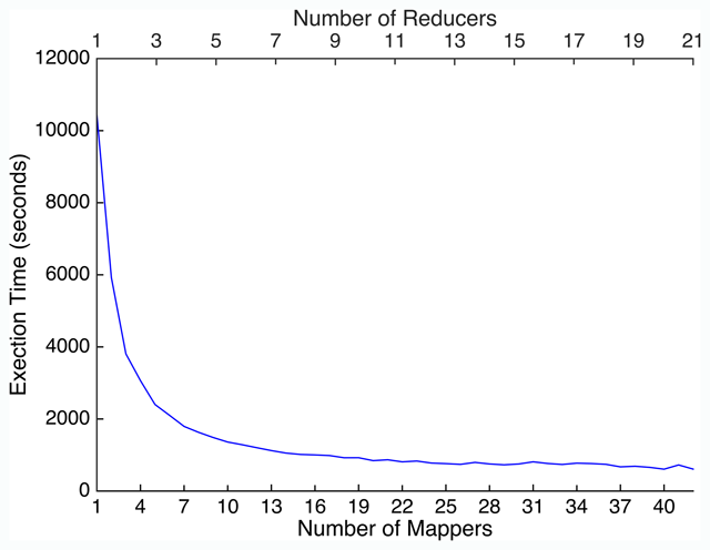
Figure 7
Execution time for the GeoSimMR using different number of mappers and reducers.
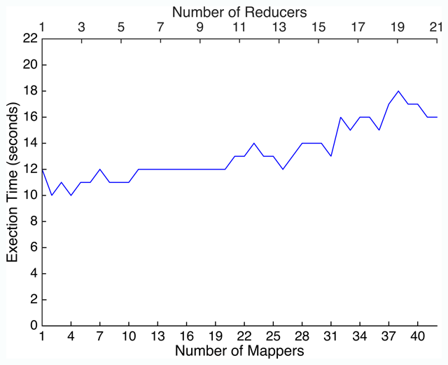
Figure 8
The execution time of the Mean Nodes Selection stage using different number of mappers and reducers.

Figure 9
The execution time of the Distances and Similarities Calculation stage using different number of mappers and reducers.
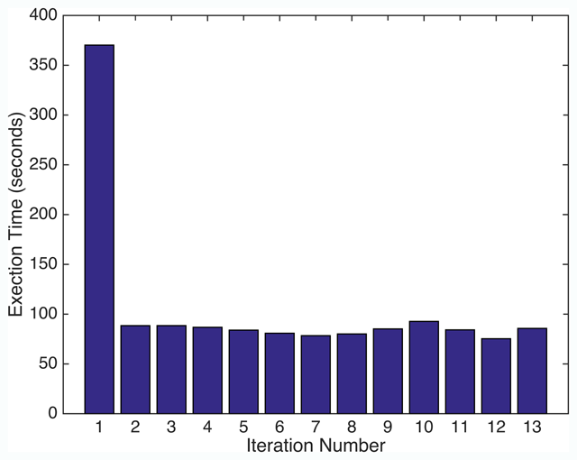
Figure 10
The execution time for every iteration of the second stage of the GeoSimMR.
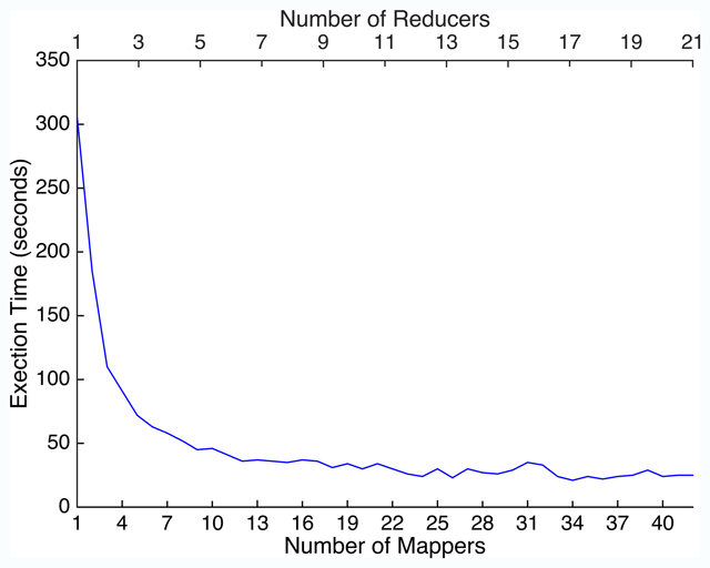
Figure 11
The execution time for the Clustering stage using different number of mappers and reducers.
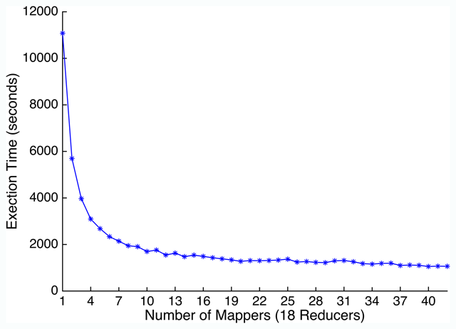
Figure 12
The overall execution time for different mappers while fixing the number of reducers.
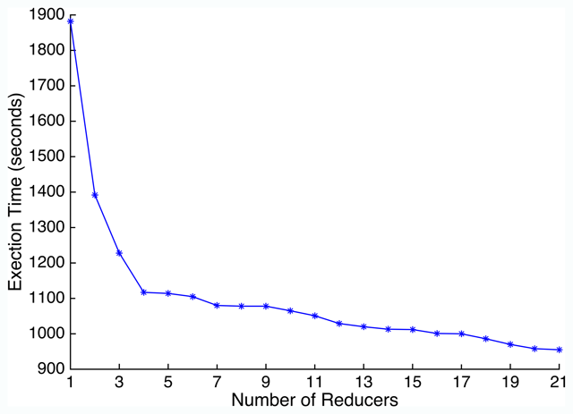
Figure 13
The overall execution time for different reducers while fixing the number of mappers to 42.

Figure 14
The overall execution time for the GeoSim and GeoSimMR using different number of nodes (Time axis is semi-log).