
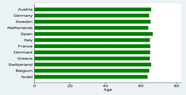
Figure 1
Key summary statistics for average age per country.
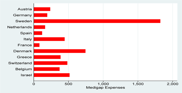
Figure 2
Key summary statistics for medigap expenses per country (%).
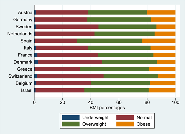
Figure 3
Key summary statistics for bmi index per country (%).
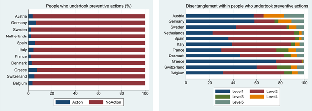
Figure 4
Key summary statistics for different level of prevention (number of preventive actions) per country (%).
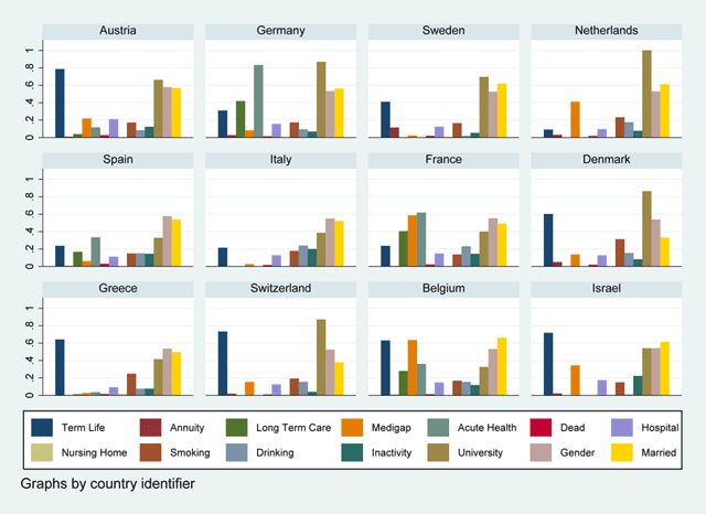
Figure 5
Key summary statistics for other variables (%).
Table 1
Relation between Insurance and Risky behaviours (Pooled Probit regression).
| Term life | Annuity | Lt care | Medigap | Acute health | ||||||
|---|---|---|---|---|---|---|---|---|---|---|
| No | Yes | No | Yes | No | Yes | No | Yes | No | Yes | |
| Main Smoking | 0.110* | 0.130** | 0.0389 | 0.0276 | –0.296*** | –0.277*** | –0.103 | –0.138 | –0.0322 | –0.0308 |
| (2.37) | (3.25) | (0.37) | (0.29) | (–5.43) | (–4.25) | (–1.08) | (–1.94) | (–0.49) | (–0.65) | |
| Drinking | –0.285*** | –0.310*** | –0.0729 | –0.0678 | –0.175 | –0.286 | 0.241 | 0.243 | –0.387*** | –0.389** |
| (–4.25) | (–5.28) | (–0.68) | (–0.66) | (–1.15) | (–1.88) | (1.43) | (1.87) | (–3.44) | (–3.26) | |
| BMI | 0.0283 | 0.0122 | –0.115** | –0.116 | –0.0138 | –0.114 | –0.151*** | –0.154*** | –0.311*** | –0.311*** |
| (0.59) | (0.23) | (–2.62) | (–1.91) | (–0.16) | (–1.70) | (–4.28) | (–3.33) | (–4.40) | (–4.70) | |
| Preventive | –0.0431 | –0.0363 | –0.100** | –0.110*** | 0.139 | 0.183 | –0.0598 | –0.0525 | 0.189** | 0.189** |
| (–1.17) | (–1.06) | (–3.25) | (–4.47) | (1.52) | (1.53) | (–1.37) | (–1.29) | (3.03) | (2.75) | |
| Inactivity | –0.179 | –0.215 | –0.408*** | –0.468*** | –0.716* | –0.819** | –0.146 | –0.0985 | –0.0624 | –0.0683 |
| (–0.97) | (–1.50) | (–7.19) | (–6.72) | (–2.13) | (–3.07) | (–1.49) | (–1.73) | (–0.62) | (–0.36) | |
| N | 2657 | 2657 | 22221 | 22221 | 1269 | 1269 | 22233 | 22233 | 1269 | 1269 |
[i] There are two different regressions for each variable: on the left the unconstrained one, while on the right the one controlled for covariates.
*p < 0.05, **p < 0.01, ***p < 0.001.
Table 2
Relation between Risk occurrence and Risky behaviours (Pooled LPM regression).
| Dead | Alive | Nursing Home | Medigap Exp | Hospital | ||||||
|---|---|---|---|---|---|---|---|---|---|---|
| No | Yes | No | Yes | No | Yes | No | Yes | No | Yes | |
| Smoking | –0.00399 | 0.00529* | –0.0217 | –0.0285 | –0.00198 | –0.000663 | –56.18 | –8.348 | –0.0223** | –0.0238*** |
| (–1.86) | (2.47) | (–1.33) | (–1.84) | (–1.42) | (–0.42) | (–1.20) | (–0.31) | (–3.92) | (–4.64) | |
| Drinking | 0.00745 | 0.0000605 | 0.0507 | 0.0483 | –0.00166 | –0.00272 | –45.09 | –42.96 | –0.00409 | –0.00232 |
| (1.87) | (0.01) | (1.87) | (1.93) | (–1.05) | (–1.23) | (–1.66) | (–1.28) | (–0.60) | (–0.29) | |
| BMI | –0.00285 | –0.00398 | 0.0202** | 0.0161** | –0.000794 | –0.000787 | –77.96 | –71.38 | 0.00773 | 0.00825 |
| (–0.88) | (–1.00) | (3.88) | (3.17) | (–0.42) | (–0.44) | (–0.96) | (–0.88) | (0.84) | (0.89) | |
| Preventive | 0.00267 | 0.00301 | –0.000823 | 0.00228 | –0.000145 | –0.000224 | –6.056 | –16.64 | 0.0262*** | 0.0260*** |
| (0.72) | (1.20) | (–0.11) | (0.29) | (–0.10) | (–0.16) | (–0.39) | (–1.08) | (9.14) | (8.91) | |
| Inactivity | 0.0777*** | 0.0635*** | –0.103* | –0.0841* | 0.0164 | 0.0151 | 253.3** | 190.1** | 0.169*** | 0.173*** |
| (12.06) | (10.11) | (–3.08) | (–2.68) | (1.81) | (1.90) | (4.05) | (3.93) | (17.17) | (13.96) | |
| N | 22233 | 22233 | 22233 | 22233 | 15040 | 15040 | 22233 | 22233 | 22226 | 22226 |
[i] There are two different regressions for each variable: on the left the unconstrained one, while on the right the one controlled for covariates.
*p < 0.05, **p < 0.01, ***p < 0.001.
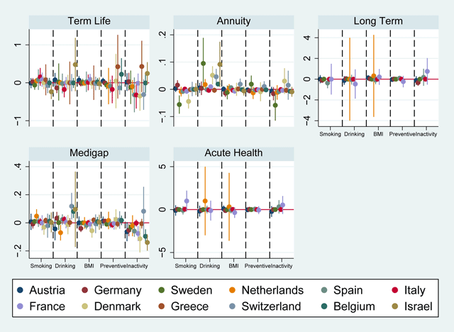
Figure 6
Relation between Insurance and Risky behaviours (LPM regression) per country.
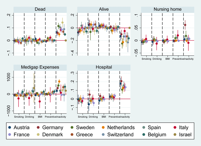
Figure 7
Relation between Risk occurrence and Risky behaviours (LPM regression) per country.
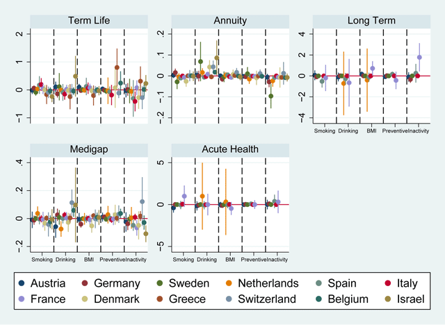
Figure 8
Relation between Insurance and Risky behaviours (LPM regression) per country with control variables.
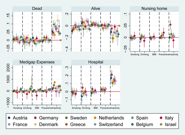
Figure 9
Relation between Risk occurrence and Risky behaviours (LPM regression) per country with control variables.
Table 3
Relation between Insurance and Risky behaviours with fixed-effect (Probit regression).
| Term life | Annuity | Lt care | Medigap | Acute health | ||||||
|---|---|---|---|---|---|---|---|---|---|---|
| No | Yes | No | Yes | No | Yes | No | Yes | No | Yes | |
| Main Smoking | 0.0947* | 0.120** | –0.00152 | 0.0190 | –0.347*** | –0.315*** | 0.0218 | –0.0340 | 0.0961 | 0.0445 |
| (2.40) | (2.70) | (–0.01) | (0.18) | (–5.78) | (–3.99) | (0.86) | (–1.68) | (1.29) | (0.70) | |
| Drinking | –0.194 | –0.227* | 0.161 | 0.0964 | 0.0955* | –0.0229 | 0.0988* | 0.0764 | –0.0981 | –0.0613 |
| (–1.76) | (–2.22) | (1.68) | (0.98) | (2.23) | (–0.33) | (2.00) | (1.74) | (–0.68) | (–0.37) | |
| BMI | 0.0435 | 0.0270 | –0.123 | –0.128 | 0.0999* | –0.00520 | –0.0804 | –0.0709 | –0.459*** | –0.464*** |
| (0.83) | (0.50) | (–1.90) | (–1.87) | (2.48) | (–0.12) | (–1.81) | (–1.49) | (–13.05) | (–14.13) | |
| Preventive | –0.0428 | –0.0376 | –0.111** | –0.104*** | 0.0757 | 0.102 | 0.0229 | 0.0337 | 0.150*** | 0.138** |
| (–1.18) | (–1.31) | (–3.10) | (–3.59) | (1.33) | (1.38) | (0.87) | (1.75) | (3.38) | (2.96) | |
| Inactivity | –0.193 | –0.241 | –0.290*** | –0.426*** | –0.835** | –0.890** | –0.234*** | –0.140* | 0.113 | 0.333*** |
| (–1.03) | (–1.58) | (–4.98) | (–5.02) | (–2.65) | (–3.12) | (–4.49) | (–2.38) | (0.79) | (3.53) | |
| N | 2657 | 2657 | 22221 | 22221 | 332 | 332 | 22233 | 22233 | 390 | 390 |
[i] There are two different regressions for each variable: on the left the unconstrained one, while on the right the one controlled for covariates.
*p < 0.05, **p < 0.01, ***p < 0.001.
Table 4
Relation between Risk occurrence and Risky behaviours with fixed-effect (LPM regression).
| Dead | Alive | Nursing Home | Medigap Exp | Hospital | ||||||
|---|---|---|---|---|---|---|---|---|---|---|
| No | Yes | No | Yes | No | Yes | No | Yes | No | Yes | |
| Smoking | –0.00379 | 0.00536* | –0.0232 | –0.0344* | –0.00285* | –0.00141 | –67.52 | –20.02 | –0.0205** | –0.0200** |
| (–1.75) | (2.65) | (–1.60) | (–2.33) | (–2.76) | (–1.21) | (–1.66) | (–0.72) | (–4.08) | (–4.18) | |
| Drinking | 0.00629 | –0.00132 | 0.0212 | 0.0279 | 0.000407 | –0.000893 | –70.66 | –76.88 | 0.00319 | 0.00362 |
| (1.29) | (–0.25) | (1.31) | (1.46) | (0.31) | (–0.48) | (–1.28) | (–1.32) | (0.31) | (0.36) | |
| BMI | –0.00290 | –0.00383 | 0.0248*** | 0.0235*** | –0.00106 | –0.00121 | –82.38 | –71.16 | 0.00858 | 0.00831 |
| (–0.84) | (–0.95) | (8.55) | (6.04) | (–0.57) | (–0.70) | (–1.01) | (–0.91) | (1.05) | (0.97) | |
| Preventive | 0.00268 | 0.00300 | 0.00378 | 0.00498 | –0.000324 | –0.000322 | –4.803 | –15.51 | 0.0248*** | 0.0247*** |
| (0.74) | (1.21) | (0.42) | (0.65) | (–0.21) | (–0.23) | (–0.38) | (–1.11) | (9.41) | (9.56) | |
| Inactivity | 0.0780*** | 0.0639*** | –0.107*** | –0.0757** | 0.0183 | 0.0164 | 201.2* | 141.7 | 0.173*** | 0.172*** |
| (11.91) | (9.88) | (–5.18) | (–3.37) | (1.97) | (2.06) | (3.03) | (2.12) | (13.38) | (12.98) | |
| N | 22233 | 22233 | 22233 | 22233 | 15040 | 15040 | 22233 | 22233 | 22226 | 22226 |
[i] There are two different regressions for each variable: on the left the unconstrained one, while on the right the one controlled for covariates.
*p < 0.05, **p < 0.01, ***p < 0.001.