
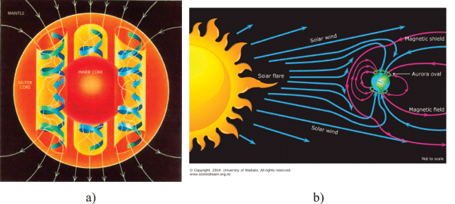
Figure 1
a) Internal sources of the Earth’s magnetic field (the axis of rotation is vertical and centered in the image) (Bloxham & Gubbins 1989). b) Solar wind plasma and the Earth’s magnetosphere (not in scale) (University of Waikato 2014).
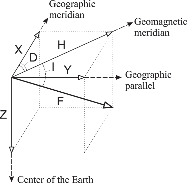
Figure 2
Decomposition of the geomagnetic field vector using the Cartesian (X, Y, Z), cylindrical (D, H, Z) and spherical (D, I, F) coordinate systems (Soloviev et al. 2013b).
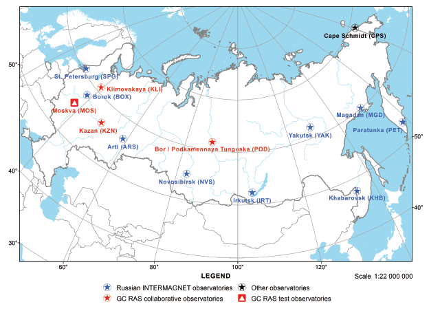
Figure 3
Map of the Russian geomagnetic observatory network. The 14 observatories that transfer geomagnetic data to the HSS: blue stars – INTERMAGNET observatories, red stars – GC RAS collaborative observatories, black stars – other observatories. The ‘Moscow’ observatory is used as a testing ground for educational and experimental purposes.
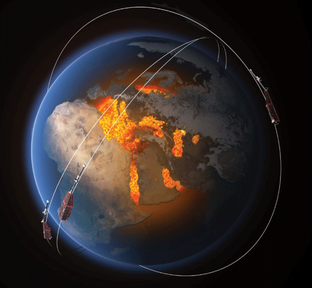
Figure 4
The Swarm constellation (not in scale) (Haagmans, Bock & Rider 2013).
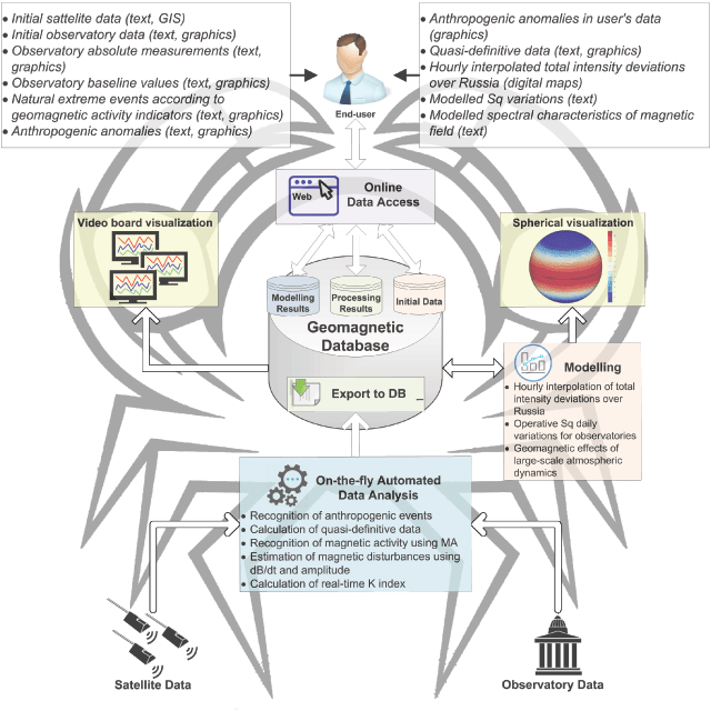
Figure 5
Data flow within the HSS.
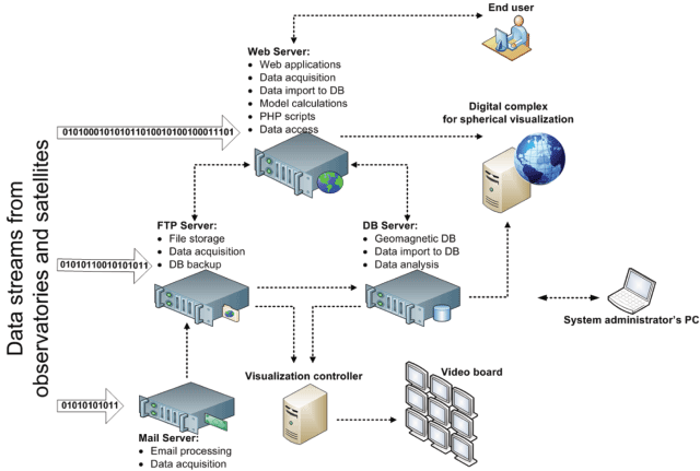
Figure 6
HSS components, their functions, and interaction.
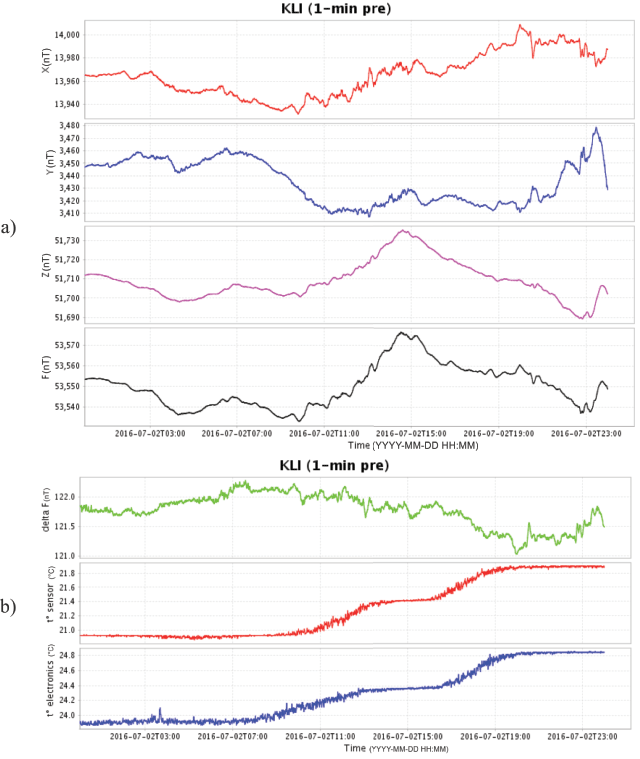
Figure 7
Magnetograms, registered at ‘Klimovskaya’ observatory: a) 1-minute magnetograms of the geomagnetic vector orthogonal components (X, Y, Z) and its measured total intensity (F); b) difference (delta F) between the measured (Fs) and calculated (Fv) values of the geomagnetic vector total intensity; temperature variations of the observatory variometer sensor (t° sensor) and electronical unit (t° electronics). The plots are generated, using the HSS data plotting tool.
Table 1
Testing DB with table for storing 1-second data, which contains 400 million random values.
| Criterion | No grouping | Daily grouping | Hourly grouping |
|---|---|---|---|
| Access speed (daily data), s | 2.0 | 0.25 | 0.1 |
| DB volume, GB | 16.3 | 3.72 | 3.72 |
| Index volume, GB | 7.36 | 0 | 0.001 |
| Record length, KB | 0.03 | 1097 | 46 |
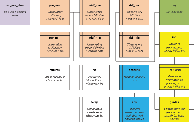
Figure 8
Scheme of the geomagnetic DB tables for storing initial ground and satellite geomagnetic data and their processing results. Tables with orange filling refer to initial observatory data, blue – to absolute observatory data, violet – to initial satellite data, green – to modelling results and yellow – to geomagnetic activity indicators.
Figure 9
Example of recognition of anthropogenic spikes in the incoming data. Purple line: 1-minute geomagnetic data (Z component). Recognized spikes are marked with black. Observatory ‘Arti’.
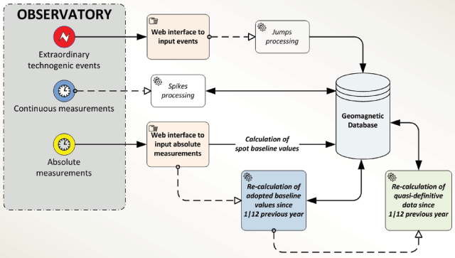
Figure 10
The HSS automated unit for calculation of the quasi-definitive geomagnetic data within the ‘Data analysis’ module of the HSS.
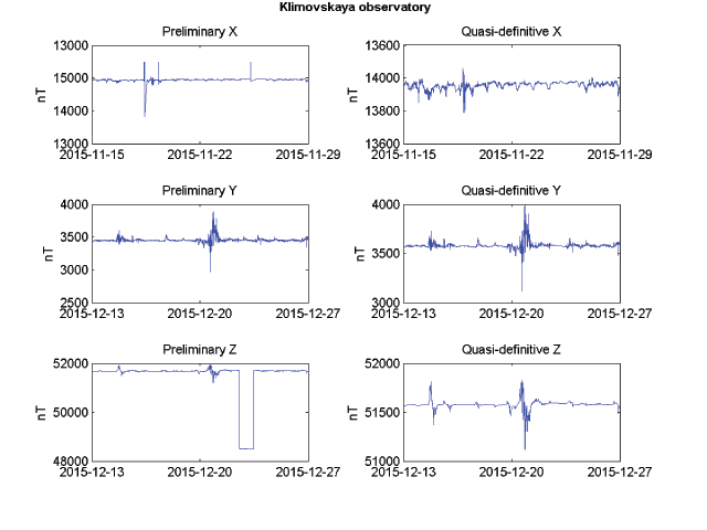
Figure 11
Preliminary and quasi-definitive magnetograms for the ‘Klimovskaya’ observatory for the period 01.11.2015–31.12.2015. The preliminary magnetograms of the three components demonstrate the following disturbances: X-component – spikes; Y-component – scale factor change; Z-component – jumps.
Table 2
The indicators of natural geomagnetic activity: time resolution and resulting values.
| Indicator | Time interval | Resulting values |
|---|---|---|
| MA | 1 minute | Value of the measure of anomality for each of the geomagnetic vector components (X, Y, Z, F or H, D, Z, F) for a 1-minute time interval |
| dBdt | 1 hour; 3 hours | Maximal value of the rate of change for each of the geomagnetic vector components (X, Y, Z, F or H, D, Z, F) within the corresponding time interval |
| Amp | 1 hour; 3 hours; 1 day | Maximal value of disturbance amplitude for each of the geomagnetic vector components (X, Y, Z, F or H, D, Z, F) within the corresponding time interval |
| Kind | 10 minutes; 3 hours | K-index values for the corresponding time intervals |
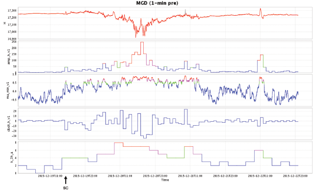
Figure 12
Graphical representation of H component variations (upper plot) from ‘Magadan’ observatory (MGD) and derived geomagnetic activity indicators for the period 19–22 December 2015: amp_h_v1 – Amp hourly maximum amplitudes of H values, mu_min_v1 – MA minute values based on H record, dbdt_h_v1 – dBdt hourly maximum values of the H component rate of change, k_3h_a – 3-hour K index values. Different colors in plots with geomagnetic activity indicators reflect different magnetic field conditions: blue – ‘background’, green – ‘weak anomaly’, purple – ‘anomaly’ and red – ‘strong anomaly’. Time of storm sudden commencement (SC) is marked with a vertical arrow.
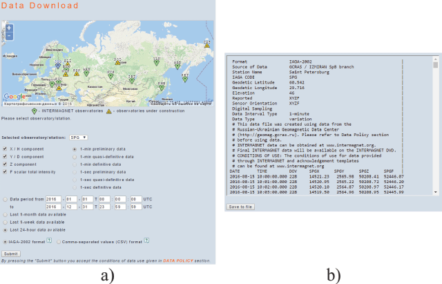
Figure 13
‘Data Access’ modules: a) web interface for online access to observatory data; b) results of a DB query in the IAGA-2002 format. Observatory ‘Saint Petersburg’.
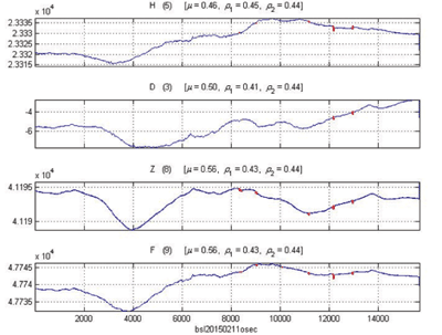
Figure 14
Results of recognition of artificial disturbances (marked with red) on user’s magnetograms (H, D, Z, F components) from observatory ‘Belsk’ (BEL), Poland.
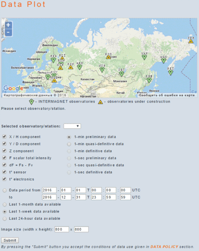
Figure 15
Web interface of the HSS online visualization of geomagnetic data.
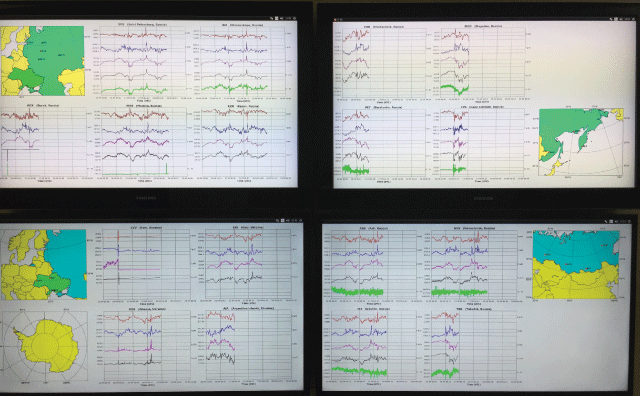
Figure 16
HSS visualization of incoming geomagnetic data from the observatories on the video board.
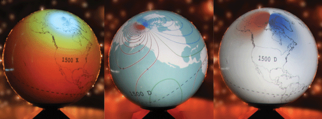
Figure 17
Visualization of geomagnetic data on a spherical screen (Berezko et al. 2011).
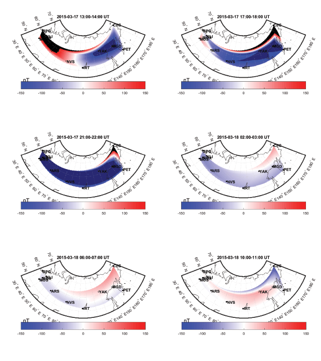
Figure 18
Visualization of interpolated hourly deviations of the total intensity of geomagnetic field for the territory of Russia during the main and recovery phases of the magnetic storm of 17–18 March 2015 (2015-03-17 13:00–2015-03-18 08:00 UT). Interpolation is performed for the region, provided with observatory measurements.
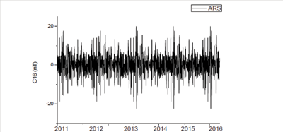
Figure 19
Time series of the amplitude of oscillating 16-day modes in the H geomagnetic component at observatory ‘Arti’ in January 2011–March 2016.