
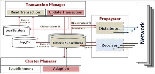
Figure 1
System Node Components.
Algorithm 1
Identifying Object subscribers.
| Inputs → Log matrix(OT), total number of nodes (N), total number of objects (O), CC[N][N] |
|---|
| For each row ∈ OT do using counter i: deadline[OT.objectID][OT.Node]= min (VD[i],DL[i]) |
| loop |
| Set Boolean matrix:Subscribers [nodes][objects][nodes] ← false; |
| For each row ∈ deadline[O][N] using iterator (i) do: |
| Set ObjectID ← i |
| Set counter C ← 0 |
| For each col ← deadline[o][N] using iterator j |
| IF (deadline[i][j] ≠ Φ) then |
| set VD= deadline[i][j]; set NodeID =j; |
| set temp[C++] ← NodeID; // temporary structure |
| End if |
| Loop |
| For x from 0 to C−2 |
| For iterator y from x+1 to C−1 |
| IF CC[temp[x]][temp[y]]<VD then |
| Subscribers[temp[x]][ObjectID][temp[y]] ← True; |
| Subscribers[temp[y]][ObjectID][temp[x]] ← True; |
| End if |
| loop |
| loop |
| loop |
| Outputs → Subscribers[N][O][N] |
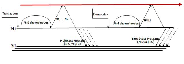
Figure 2
Distributor (publisher) module.
Algorithm 2
Rep-read(O): Retrieving recent information.
| Inputs → data object identifier ObjectID |
|---|
| Set O ← Object_ID |
| Set i ← 0 |
| Temp[][] ← ø |
| For each row ∈ Rep_dir[][Object_ID] do |
| If Rep_dir[row][ ObjectID]= O then |
| Temp[i][value] = Rep_dir[row][ value] |
| Temp[i][TS] = Rep_dir[row][TS] |
| Break; |
| End if |
| i ← i + 1 |
| Loop |
| sort(temp) on TS descending |
| Object_recent[value] ← Temp[i][value] |
| Object_recent[TS] ← Temp[i][TS] |
| outputs → Temp[i][TS] & Temp[i][value] of most recent value of ObjectID |
Algorithm 3
On-demand Read Transactions.
| Inputs → Object Id (O) |
|---|
| //Read object’s value and timestamp from local database |
| Set SrcState ← Object_value |
| Set SrcTS ← Object_ TS |
| //Read object’s value and timestamp from Rep_dir in |
| Set RState ← Rep_read.get(value) |
| Set RTS ← Rep_read.get(TS) |
| IF RTS<SrcTSthen // less recent |
| State ← RStateelse State |
| Else State ← SrcState |
| End IF |
| //Update local value of to Object_Id V |
| Local_Database [Object_Id][value] ← State |
| Return(State) |
| Outputs → value for (O) |
Table 1
Experiment settings.
| Parameter | Default value |
|---|---|
| # Nodes | 10 |
| Database size | 100 objects/node |
| Data size | 64 byte |
| Validity interval | 1−2.8 sec |
| Transaction size | 5 update operations |
| Transaction arrival time | [200–1,000] |
Table 2
Number of write operations generated in each node.
| Node | N1 | N2 | N3 | N4 | N5 | N6 | N7 | N8 | N9 | N10 | total |
|---|---|---|---|---|---|---|---|---|---|---|---|
| Workload 1 | 21 | 23 | 26 | 22 | 30 | 43 | 40 | 43 | 41 | 30 | 319 |
| Workload 2 | 101 | 103 | 106 | 102 | 110 | 123 | 120 | 123 | 121 | 111 | 1,120 |
Table 3
Storage Cost Evaluation of the proposed protocol.
| Cluster Capacity | 2 | 3 | 4 | 5 | 6 | Full |
|---|---|---|---|---|---|---|
| Storage cost | 128 | 192 | 256 | 320 | 384 | 640 |
Table 4
Number of migration objects (transmitted messages).
| # write operations | # migration objects | ||
|---|---|---|---|
| Proposed work | DYFRAM | ||
| Workload 1 | 984 | 620 | 1,385 |
| Workload 2 | 4,008 | 1,081 | 3,173 |
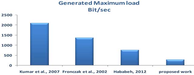
Figure 3
Maximum Load Evaluation.
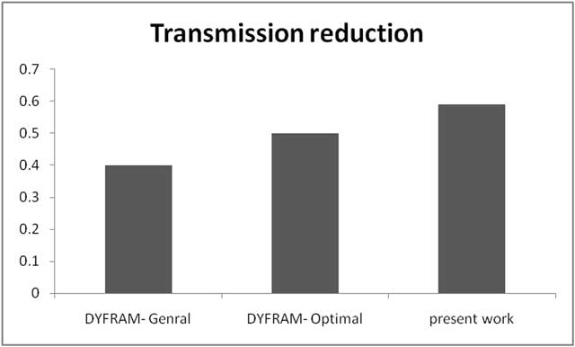
Figure 4
Comparative Evaluation with DYFRAMA.
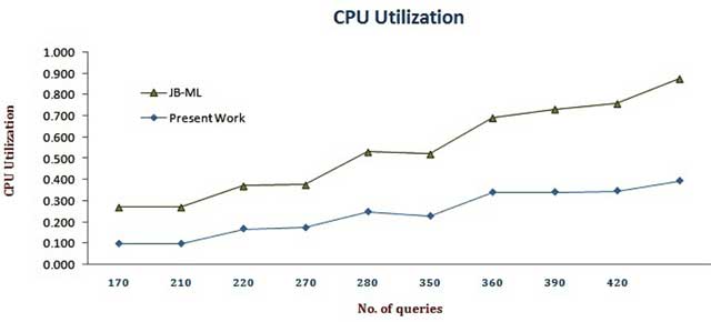
Figure 5
CPU utilization of present work.
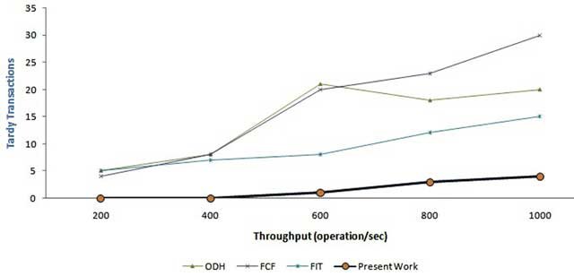
Figure 6
Comparative evaluation from the proposed protocol and other works.