
1. Introduction
Prostate cancer is the second most commonly diagnosed cancer among men worldwide and one of the leading causes of cancer-related mortality in the male population. Its treatment poses a serious challenge [1]. Conventional therapeutic approaches include prostatectomy, radiotherapy, hormone therapy, and chemotherapy. Although these treatments are widely used in clinical practice, they are often associated with substantial side effects and do not always provide satisfactory therapeutic outcomes, particularly in advanced stages of the disease. Consequently, the development of new therapeutic strategies that are both effective and minimally invasive remains an important research objective [2,3].
One of the promising therapeutic approaches currently investigated is hyperthermia therapy, which involves controlled heating of tumour tissue to temperatures typically ranging from 42 to 45°C. At these temperatures, cancer cells become more susceptible to thermal damage and apoptosis, while normal tissues can tolerate such thermal exposure for limited periods of time. Furthermore, hyperthermia has been shown to significantly enhance the effectiveness of other therapeutic modalities such as radiotherapy and chemotherapy by improving tumour perfusion and oxygenation and by increasing the sensitivity of cancer cells to radiation and cytotoxic drugs [4].
Among the different hyperthermia techniques, magnetic hyperthermia has attracted considerable attention due to its ability to generate localized heating within tumour tissue using magnetic nanoparticles exposed to an alternating magnetic field. In this method, magnetic nanoparticles are introduced into the tumour region and subsequently subjected to an external alternating magnetic field, which leads to the dissipation of electromagnetic energy in the form of heat [5]. This approach enables relatively precise control of heat generation within the targeted region and therefore may significantly reduce damage to surrounding healthy tissues.
The mechanism of heat generation in magnetic nanoparticles is mainly related to magnetic relaxation processes occurring within the particles. Two primary mechanisms are responsible for this phenomenon: Néel relaxation and Brownian relaxation. Néel relaxation involves the reorientation of the magnetic moment inside the nanoparticle without physical rotation of the particle itself, whereas Brownian relaxation is associated with the rotational motion of the entire nanoparticle in a viscous medium [6,7]. The effective relaxation time of the nanoparticles is determined by the combined contribution of these mechanisms and represents a key parameter influencing the heating efficiency of magnetic nanoparticles in alternating magnetic fields [8,9].
The heating efficiency of magnetic nanoparticles is typically characterized by the volumetric power density P. It depends on several factors, including the amplitude and frequency of the applied magnetic field as well as the magnetic and physical properties of the nanoparticles. Parameters such as particle size and the viscosity of the surrounding medium strongly influence the magnetic relaxation processes and therefore affect the heat generation capability of the nanoparticles [5,10]. Optimization of these parameters is essential for achieving efficient heating while maintaining safe exposure conditions for patients.
Another important factor affecting the temperature distribution during hyperthermia therapy is the geometry and volume of the heated region. The shape and size of the tumour influence heat transfer and thermal dissipation within biological tissues, which in turn affect the temperature achieved during treatment. Therefore, the concentration of magnetic nanoparticles required to obtain therapeutic temperatures may vary depending on the geometry of the treated region. Numerical modelling and computational simulations are widely used to analyse such effects and to optimize treatment parameters prior to clinical applications [11,12].
Although numerous studies have focused on the magnetic properties of nanoparticles and the influence of magnetic field parameters on heating efficiency, relatively little attention has been devoted to the influence of tumour geometry on the concentration of nanoparticles required to achieve therapeutic temperatures. Most studies assume simplified tumour geometries or focus primarily on nanoparticle properties, while the influence of the size and shape of the heated region on the required nanoparticle concentration is less frequently analysed [13,14].
The aim of this study was therefore to determine the concentration of magnetic nanoparticles required to achieve therapeutic temperatures in prostate cancer treatment using magnetic hyperthermia, taking into account the influence of the geometry and volume of the heated region. An air coil generating an alternating magnetic field was developed to obtain a uniform electromagnetic field distribution in the prostate region. Numerical simulations were performed using the Sim4Life software [15] for a prostate tumour and three simplified geometric models: a cylinder, a sphere, and a cube. Heat generation by magnetic nanoparticles was calculated using the theoretical model proposed by Rosensweig [6], which enabled the estimation of the nanoparticle concentration required to achieve the therapeutic temperature.
2. Materials and methods
2.1. Numerical model of the electromagnetic field
The electromagnetic field distribution was calculated using the magneto-quasi-static formulation implemented in the simulation environment. In this approach, the electromagnetic field was described by the following equation:
where σ is the electric conductivity, ϕ stands for the electric scalar potential, ω represents the angular frequency, and A is the magnetic vector potential. The equation was considered together with a zero Neumann boundary condition, which corresponds to a vanishing normal current flux at the boundaries of the computational domain.The simulations were performed using a real-valued solver. The electric field (E-field) was calculated only within the lossy (σ ≠ 0) regions of the model, while the magnetic field (H-field) was evaluated throughout the entire computational domain. Consequently, the numerical grid was defined primarily within the lossy domain where energy dissipation occurs. The external electromagnetic excitation generated by the coil was expressed using the vector potential formulation. The E-field was obtained from the vector potential using tricubic interpolation, while the magnetic flux density was used to determine both the magnetic field intensity and the magnetic flux density distributions [15].
If the vector potential is not explicitly defined, it can be calculated using the Biot–Savart law:
where J 0 is the current density vector and the H-field can be expressed as:This formula allows the magnetic field generated by the current-carrying coil to be determined. In this case, the low-frequency current sources must remain outside the lossy computational domain in order to avoid numerical singularities in the field calculations [15].In magnetic hyperthermia, when magnetic nanoparticles are exposed to an H-field, magnetic power losses are generated according to the following formula [6]:
where f is the frequency, and H represents the magnetic field strength amplitude. The imaginary part of the magnetic susceptibility χ″ can be calculated according to the equation [6]:where χ 0 is the field-dependent susceptibility and ɷ stands for the angular frequency (ɷ = 2πf). The effective relaxation time τ eff may be described by the formula:where τ B is the Brownian relaxation time, τ N is the Neel relaxation time defined as follows: and η is the viscosity, k B stands for the Boltzmann constant (k B = 1.38·10−23 JK−1), T is the absolute temperature. V H represents the hydrodynamic volume of the particle and is given by:where δ represents the surfactant layer thickness, V M is the magnetic volume of magnetic nanoparticles with radius R M, and K is the anisotropy constant of the magnetic material.Susceptibility used in equation (5) is defined as:
where χ i is the initial susceptibility and can be calculated from the formula:where φ is the concentration of magnetic nanoparticles, and M d is the domain magnetization of the suspended particles. Langevin parameter ξ used in equation (11) is expressed as:2.2. Thermal simulations
The thermal simulations were based on the solution of the heat transfer equation, which describes temperature evolution in biological tissues. Heat transport in the tissue was modelled using the Pennes bioheat equation, which accounts for thermal conduction, blood perfusion, and metabolic heat generation [16]:
where T is the tissue temperature, ρ and c denote the density and specific heat of the tissue, and k is the thermal conductivity. The term Q perf represents heat exchange due to blood perfusion, Q met is the metabolic heat generation, and P represents the external heat source.To include heat exchange between the skin and the external environment, the Robin’s boundary condition was applied as follows:
where k is the thermal conductivity of the skin, h is the heat transfer coefficient, and T ext is the external temperature [17].Thermal calculations were performed using the structured-grid time-domain solver, which applies a finite-difference time-domain scheme on non-uniform grids. This approach allows efficient computation of temperature distributions while enabling local grid refinement in regions of particular interest. Electromagnetic heat sources obtained from the electromagnetic simulations were interpolated onto the thermal grid.
The voxel-based discretization enables simulations with a large number of computational cells, where each voxel can be assigned individual material parameters. This makes the method particularly suitable for modelling heterogeneous biological structures [15].
Taking into account the aforementioned mathematical models for the electromagnetic field and heat transfer, the following steps were performed. First, magnetic field H was obtained using equation (3), and then, the volumetric power density distribution was calculated using equation (4). In this way, the value of χ′′ was determined at the considered frequency. Next, the Brownian and Néel relaxation times were calculated equations (7) and (8) for superparamagnetic nanoparticles under the assumption that the optimization condition ωτ eff = 1 is fulfilled. Based on equations (3) and (12), the Langevin parameter was determined. The value of χ 0 was then calculated using equation (10), and χ i was obtained from equation (11). Finally, the concentrations of magnetic materials φ were determined using equation (11).
Additionally, the IT’IS Foundation tissue parameter database was used [18]. The tissue properties were recalculated for a frequency of f = 100 kHz, assuming that all modeled materials are uniform and not temperature dependent. In Table 1, only the prostate and the tumour’s dielectric properties were gathered as crucial ones for the temperature analysis.
Table 1
Thermophysical and electromagnetic properties of prostate and tumour tissue for frequency f = 100 kHz used in Pennes bioheat equation and in magneto-quasi-static solver [18]
| Tissue name | Mass density | Specific heat capacity | Thermal conductivity | HGR (W/kg) | HTR (W/m3/K) | Conductivity |
|---|---|---|---|---|---|---|
| ρ [kg/m3] | c [J/kg/K] | k [W/m/K] | σ (S/m) | |||
| Prostate | 1045.0 | 3760.0 | 0.5115 | 6.10369 | 27820.2 | 4.39·10−1 |
| Tumour | 1090.4 | 3421.2 | 0.4500 | 0.9061 | 2705.95 | 3.63·10−1 |
HGR – Heat Generation Rate per unit mass.
HTR – Heat Transfer Rate coefficient per unit volume and temperature difference.
Source: data from Baumgartner et al.
2.3. Computer modelling and simulation
An air coil with a radius of 350 mm, consisting of 27 turns made of wire with a radius of 3 mm, was designed in the Sim4Life software. The turns were spaced 11 mm apart. A human model was imported from The Computable Virtual Population [19] and positioned with its arms raised to prevent them from overheating. The position of the coil was adjusted so that the prostate gland was located at its center point, as depicted in Figure 1.
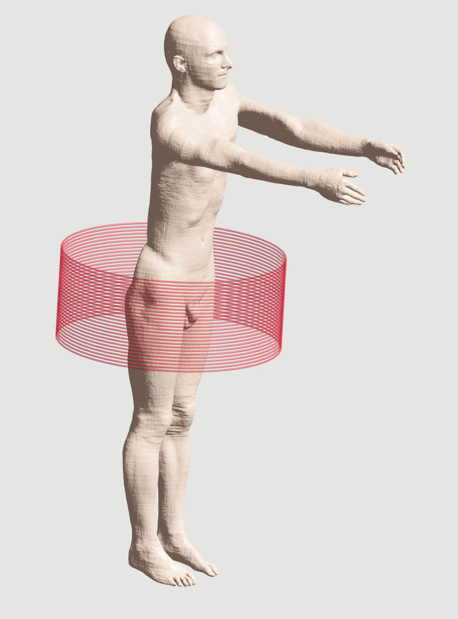
Figure 1
The designed air coil and the human model.
Magneto-quasi-static simulations were performed assuming an alternating current with an amplitude of I max = 75 A and a frequency of f = 100 kHz. For safety reasons, the parameters of the alternating magnetic field satisfied the Atkinson–Brezovich criterion, i.e. [20]. In the present study, the selected values of the magnetic field amplitude satisfy this condition, ensuring that the simulated hyperthermia treatment remains within the accepted limits for biomedical applications.
The naturalistic irregular tumour model was taken from a freely available database [21], and three geometric primitives were analyzed: a cube with a side length a = 9 mm, a cylinder with a radius r = 4 mm and a height h = 10.5 mm, and a sphere with a radius R = 5.48 mm. The dimensions of the models were selected so that the naturalistic tumour could be inserted into them (Figure 2). Volume and surface area of the geometric models are gathered in Table 2. The geometric primitives were placed in the same anatomical location within the prostate model, at the site corresponding to the location of the naturalistic tumour. In each case the electromagnetic properties of muscle tissue were assigned [14] (see Table 1).
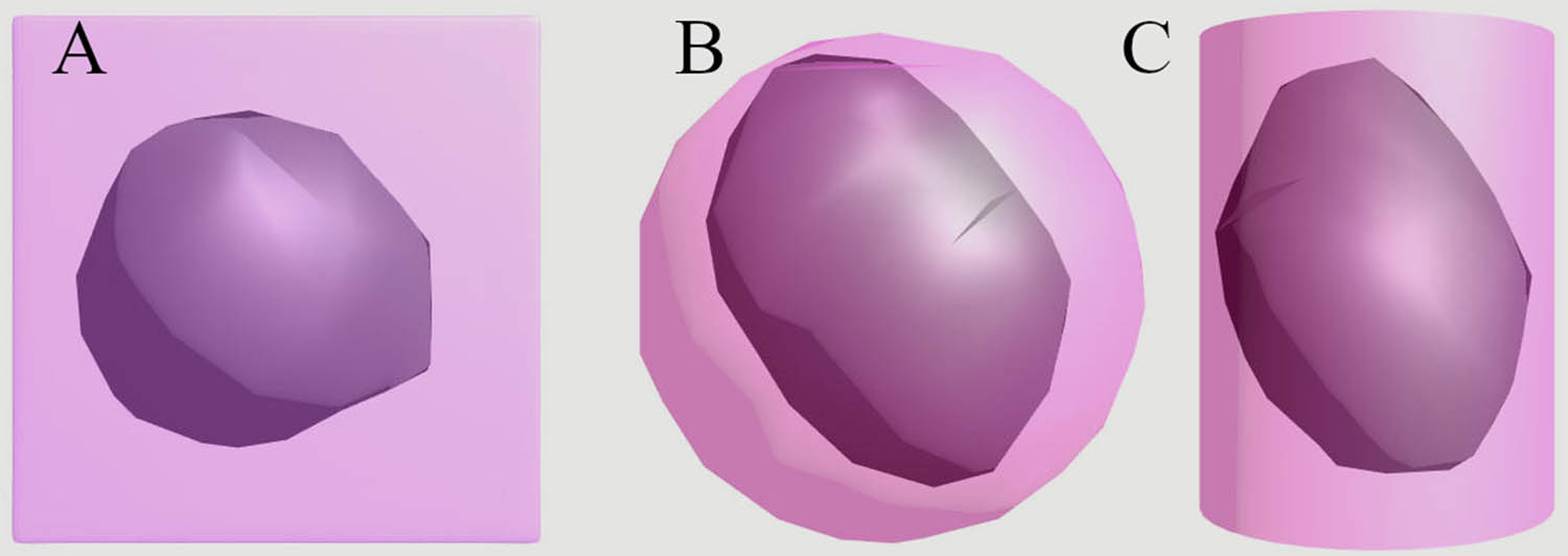
Figure 2
Comparison of geometric primitives to the naturalistic irregular tumour model: (a) cube, (b) sphere, and (c) cylinder.
Table 2
Volume and surface area of the analysed tumour models
| Tumour model | Dimensions (mm) | Volume (mm3) | Area (mm2) |
|---|---|---|---|
| Irregular | — | 392.624 | 317.599 |
| Cylinder | r = 4, h = 10.5 | 525.112 | 363.58 |
| Sphere | R = 5.48 | 689.008 | 377.971 |
| Cube | a = 9 | 728.489 | 479.669 |
As for the temperature analysis, the initial human body temperature was set to 37°C and the mixed boundary conditions were applied. The heat transfer coefficient was set to h = 5 W/m2/K, which corresponds to natural air convection [22]. In this context, the concentrations of magnetic nanoparticles φ needed to achieve the therapeutic temperature, i.e. 43–44°C were evaluated. Using the relationships described by equations (4)–(12), the concentration was determined assuming monodisperse nanoparticles (Table 3).
Table 3
Properties of magnetic nanoparticles [6]
| Magnetic material | M d (kA/m) | K (kJ/m3) |
|---|---|---|
| Maghemite | 414 | 4 |
| Magnetite | 446 | 41 |
| Cobalt ferrite | 425 | 190 |
| Barium ferrite | 380 | 315 |
Source: data from Rosensweig.
3. Results
The distributions of the magnetic field H (XY and XZ cross-sections) are shown in Figures 3 and 4, where the prostate gland is marked in white at the center. It can be seen that the prostate is located in a homogeneous magnetic field region H with a value of 2.670 kA/m.
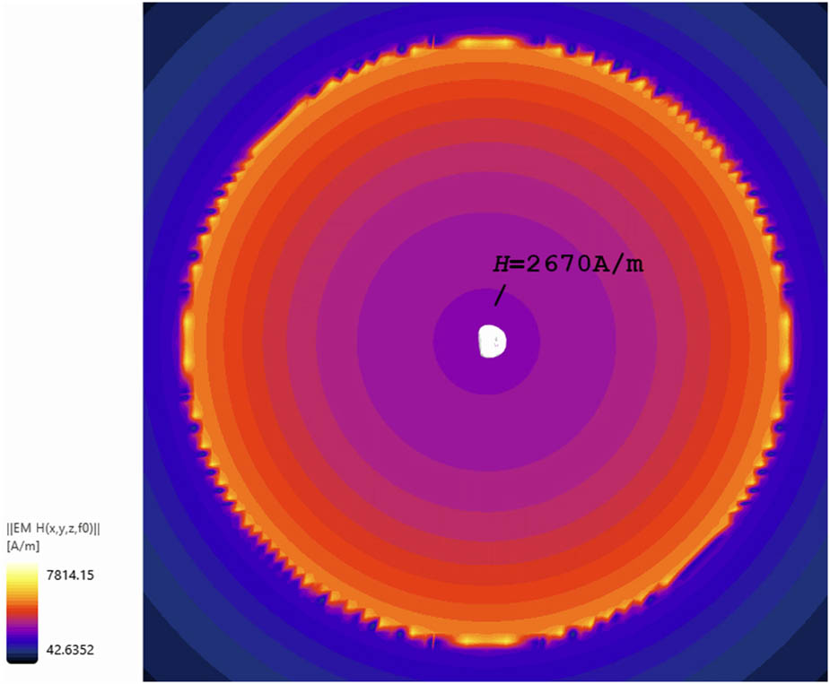
Figure 3
Magnetic field distribution (H) in the XY cross-section for f = 100 kHz with regard to the prostate (white).
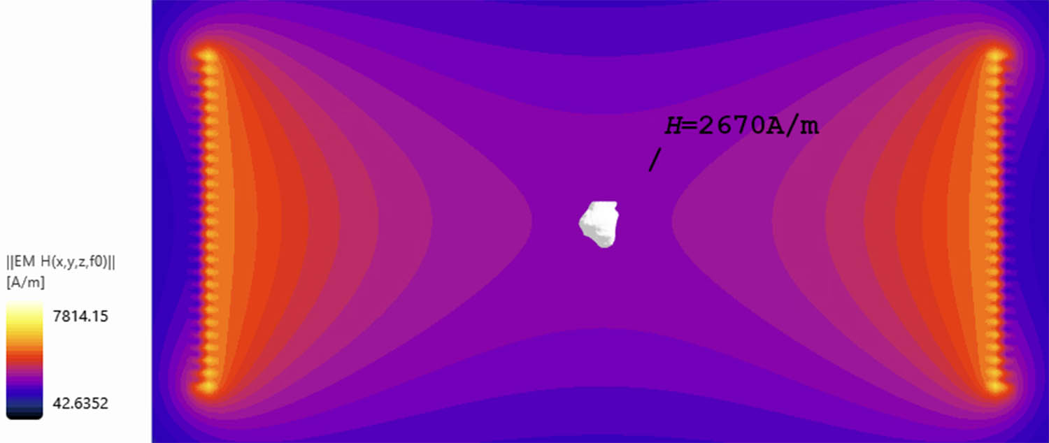
Figure 4
Magnetic field distribution (H) in the XZ cross-section for f = 100 kHz with regard to prostate (white).
In thermal simulations, the distribution of the volumetric power density P generated by magnetic nanoparticles inside the tumour models was used as the source. It was evaluated with usage of equation (4), and the calculations were performed under the assumption that ferrofluid viscosity was η = 0.0025 kg/(m·s), surfactant layer thickness was δ = 1 nm, and attempt time was τ0 = 1 ns. Considering the optimization condition ωτ eff = 1, the magnetic radius, R M, was estimated for the magnetic nanoparticles listed in Table 3. It was found that R M = 5 nm for both barium ferrite and cobalt, and R M = 13 nm for maghemite. Magnetite was excluded because the condition was not satisfied. Next, the parameters that allow achieving the therapeutic temperatures across different models regarding magnetic material were estimated (see Table 4). In the case of tumour, a power density of 712.9 kW/m3 is required to reach the therapeutic temperature; however, depending on the magnetic material, different concentrations of magnetic nanoparticles (MNPs) must be used – for example, a concentration φ = 0.44% for maghemite, 5.5% for cobalt ferrite, and 6.87% for barium ferrite.
Table 4
Comparison of magnetic nanoparticle parameters required to achieve therapeutic temperatures in different tumour models for H = 2.67 kA/m and f = 100 kHz
| Tumour model | φ (%) | Maximum power density | ||
|---|---|---|---|---|
| Maghemite | Cobalt ferrite | Barium ferrite | P (W/m3) | |
| Naturalistic | 0.489 | 5.49 | 6.87 | 712890 |
| Cylinder | 0.293 | 3.30 | 4.12 | 427734 |
| Sphere | 0.269 | 3.02 | 3.78 | 392089 |
| Cube | 0.244 | 2.75 | 3.43 | 356445 |
Figure 5 presents the distribution of power density P (XY- and XZ-cross-sections) for the analysed tumour models. The highest values are observed for the naturalistic tumour represented by the red curve, which reaches a maximum value of P of about 700 kW/m³ in the central region. Much lower values occur for the cylindrical model, where the power density stabilizes at around 430 kW/m³ across a similar range. The black curve, which represented spherical model, shows moderate values, peaking at approximately 400 kW/m³, with a more rounded profile indicating smoother transitions. The lowest power density P is recorded for the cubic model, with values around 350 kW/m³ in the center. For all models, the values decrease towards the edges and approach zero.
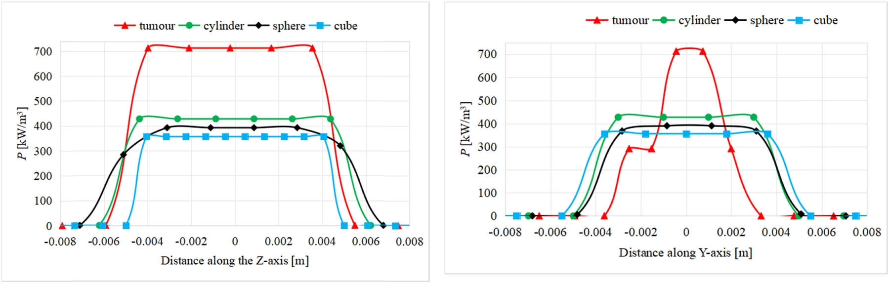
Figure 5
Volumetric power density P required to achieve therapeutic temperature in the analysed tumour models (XY cross-section (left) and XZ cross-section (right)).
In the next step, the analysis was conducted to identify differences in the temperatures obtained for the naturalistic tumour model and the primitive models. This demonstrated how the assumed tumour’s shape can influence quantitative temperature analyses. For this purpose, the power density required from MNPs to achieve the therapeutic temperature for the naturalistic tumour was taken from Table 4, and the same value was then used to calculate the temperature for the geometric primitives, i.e. for cylinder, sphere, and cube. An analogous methodology was adopted for the other cases, i.e., the power density, which is the source of the therapeutic temperature for one of the geometric primitives, was used to estimate the temperature for the other tumour models. The temperature over time for naturalistic tumour, cylindrical, spherical, and cubic models has been collected in Figure 6, where each of the tumour models was used as the reference for the others. Furthermore, it can be seen that the temperature stabilized after about 500 seconds in all tumour models, but the heating time was 60 minutes in all cases (the graphs have been shortened due to practical reasons). It should be noted that the main reason for the prolonged heating time and slow rise in temperature is the occurrence of necrosis.
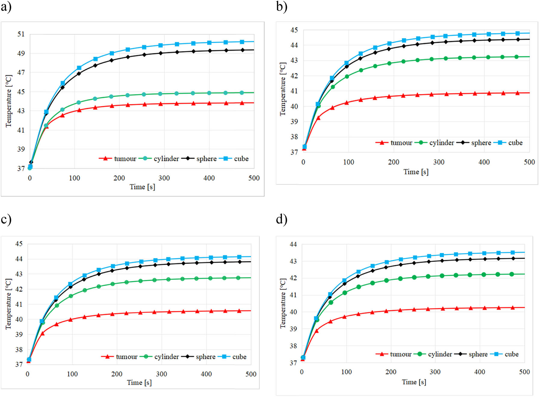
Figure 6
The temperature rise over time in analysed models regarding (a) naturalistic tumour (P = 712890 W/m3), (b) cylinder (P = 427734 W/m3), (d) sphere (P = 392089 W/m3), and (e) cube (P = 356445 W/m3).
The concentrations of magnetic materials that allowed the required temperature to be achieved in the naturalistic tumour model were as follows: for maghemite φ = 0.489%, for cobalt ferrite φ = 5.49%, and for barium ferrite φ = 6.87% (Figure 6a). The maximum value of volumetric power density was P = 713 kW/m3. In the case of other considered models, the temperature exceeded the acceptable range for the same power density.
The results shown in Figure 6b were obtained for a power density equal to P = 428 kW/m3. In this case, the cylindrical tumour model was the reference one. The concentrations of magnetic materials were as follows: for maghemite φ = 0.293%, for cobalt ferrite φ = 3.30%, and for barium ferrite φ = 4.12%. It can be seen that the temperature in the naturalistic tumour model remained below the desired range. In the cylindrical model, the temperature reached the therapeutic level. In the remaining models, the temperature exceeded the required limits.
The following values of magnetic materials enabled achieving the therapeutic temperature in the spherical model (Figure 6c): maghemite φ = 0.269%, cobalt ferrite φ = 3.02%, and barium ferrite φ = 3.78%. The maximum value of volumetric power density was equal to P = 392 kW/m3. In the naturalistic tumour model, the achieved temperature was much below the acceptable range. As in the case of the previous model, the temperature in the cylindrical model remained below the desired limits. In the cubic model, the temperature exceeded the required range.
Finally, the results shown in Figure 6d were evaluated for the cubic model as the reference. The volumetric power density was P = 356 kW/m3 and the following values of the concentrations of magnetic materials were used: for maghemite φ = 0.244%, for cobalt ferrite φ = 2.75%, and for barium ferrite φ = 3.43%. In this case, the temperature increased to the therapeutic level in the cubic and spherical models. It is worth noting that, in the other considered models, the temperature was below the acceptable range.
4. Discussion
The highest values of nanoparticle concentrations (φ) and the volumetric power density (P) are observed for the naturalistic tumour model. There, the nanoparticle concentration reaches φ = 0.489% for maghemite, φ = 5.49% for cobalt ferrite, and φ = 6.87% for barium ferrite, resulting in the highest power density P. For models such as the cylinder, sphere, and cube, the concentration φ decrease, leading to a gradual reduction in generated volumetric power P. A consistent trend can be observed across all models: larger nanoparticle concentration corresponds to increased heat generation and temperature.
It can also be observed that for spherical and cubic models, the temperature difference is the smallest, ranging from 0.5°C to 1°C relative to each other. However, when comparing the spherical and cubic models with the naturalistic model, the temperature difference is the greatest. This may mean that simplifying the tumour model to a sphere or cylinder results in the greatest discrepancies.
In the case of the cylindrical model, the obtained temperatures were always between those of the naturalistic model and the spherical and cubic models. It is worth noting that in the case of this simplification, the temperature difference was smallest when the naturalistic model served as the reference one (see Figure 6a). This may indicate that in this case, simplifying the model will result in the smallest differences in temperature estimation.
The simulations revealed that the geometry and size of the heated region significantly influence the resulting temperature distribution. When the same nanoparticle concentrations were applied to the geometric primitives, the maximum temperatures exceeded the therapeutic range. To obtain temperatures at the therapeutic level for geometric primitives, it was necessary to reduce the concentration of magnetic nanoparticles. This confirms that accurate estimation of nanoparticle concentration is essential for safe and effective hyperthermia treatment. Excessive heating could potentially damage surrounding healthy tissue.
In studies on magnetic hyperthermia, tumour regions are often simplified and represented by basic geometrical shapes such as spheres, cylinders, or cubes [23,24]. However, the results of the present simulations suggest that this approach may be inappropriate. Significant differences were observed in heat generation induced by magnetic nanoparticles between the naturalistic tumour model and simplified geometries. These discrepancies show that simplifying the geometry can lead to inaccurate predictions of temperature distribution and heating efficiency. Therefore, this approach should be used with caution when modelling magnetic hyperthermia.
It should also be noted that the simulations were performed under several simplifying assumptions, such as uniform nanoparticle distribution, monodisperse particle size, and constant thermophysical properties of the tissue. In real biological conditions, factors such as polydispersity and non-uniform nanoparticle distribution may influence the temperature distribution. Therefore, further studies, including more complex models, may improve the accuracy of the predictions.
5. Conclusions
The study showed that the geometry and size of the heated region have a significant influence on the resulting temperature distribution. When the same nanoparticle concentrations were applied to geometric primitives such as a cylinder, sphere, and cube, the obtained temperatures varied and exceeded the therapeutic range. Therefore, it was necessary to reduce the nanoparticle concentration to maintain the temperature within the desired therapeutic limits. This indicates that the concentration of magnetic nanoparticles required for effective hyperthermia treatment depends not only on the magnetic field parameters but also on the geometry and thermal properties of the heated region. The results show that simplifying tumour geometry to basic shapes may lead to significant inaccuracies in predicting heating efficiency in magnetic hyperthermia. Accurate estimation of nanoparticle concentration is therefore essential to ensure safe and controlled temperature increase during therapy.
Funding information
Authors state no funding involved.
Author contributions
A. Miaskowski Contribution: The preparation of the research program. The execution of research. The interpretation of data. Preparation of the manuscript. D. Szymańska Contribution: The execution of research. The statistical analysis. The interpretation of data. Preparation of the manuscript Ł. Fuśnik Contribution: The statistical analysis. The interpretation of data. Preparation of the manuscript Obtain financing.
Conflict of interest statement
Authors state no conflict of interest.