
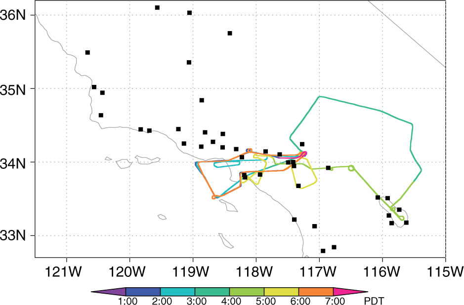
Fig. 1
Map of the surface sites (black squares) and aircraft flight track on 2 June 2010 (coloured curve). The flight started at 01:00 PDT and ended at 07:00 PDT, lasting for 6 hours. Colours indicate the flight time.
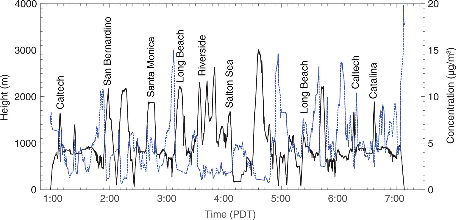
Fig. 2
Evolution of the flight height (black) and the total concentration of OC, NO3, SO4 and NH4 (blue dashed curve) along the aircraft flight track from 01:00 to 07:00 PDT 2 June 2010.
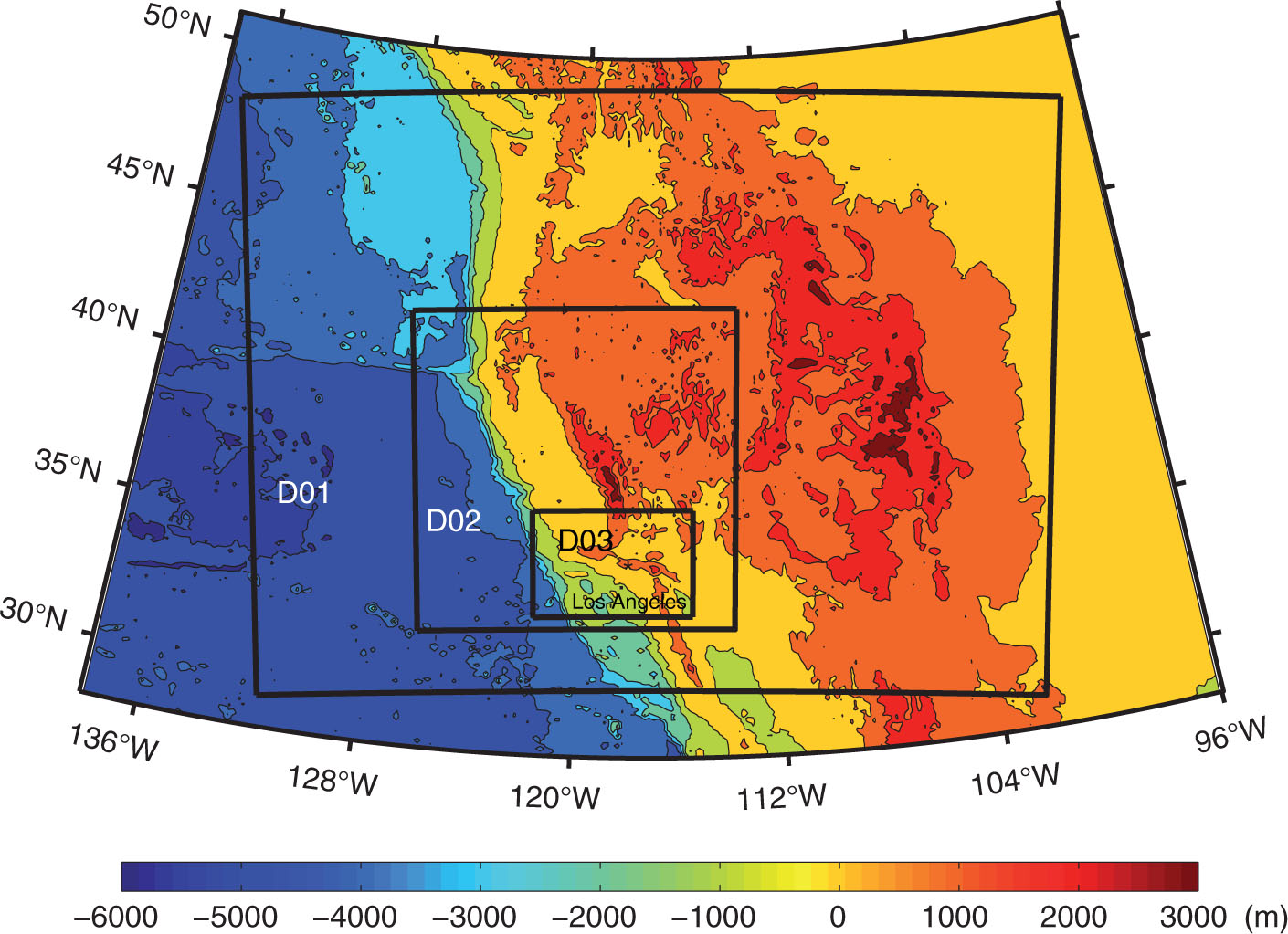
Fig. 3
Three-nested model domains. The innermost domain covers the Los Angeles basin, and the black square indicates the location of Los Angeles. Colours indicate topographic elevations.
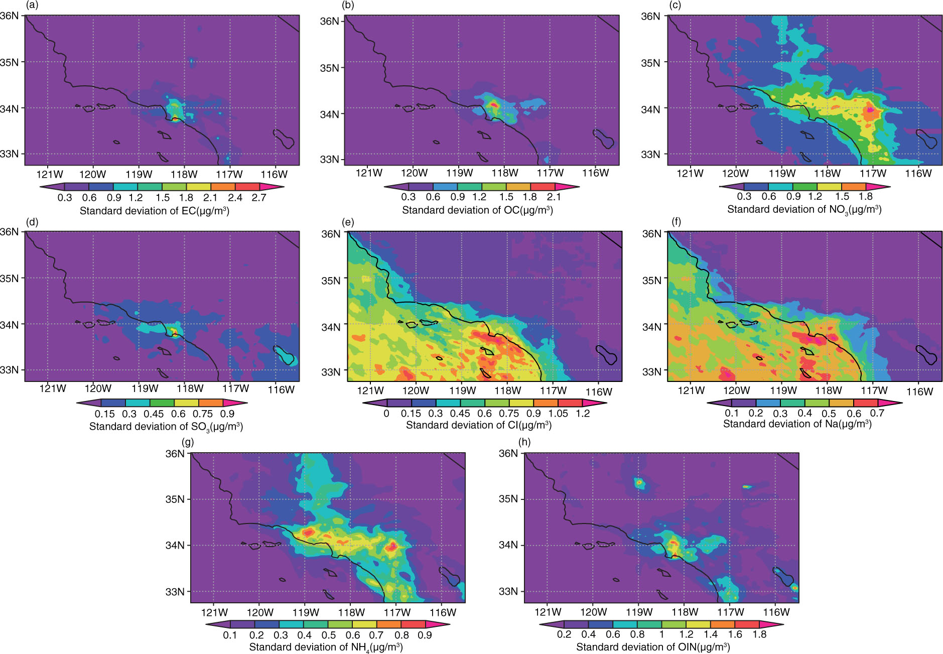
Fig. 4
Surface distribution of the SD of aerosol species of EC (a), OC (b), NO3 (c), SO4, (d), Cl (e), Na (f), NH4 (g) and OIN (h).
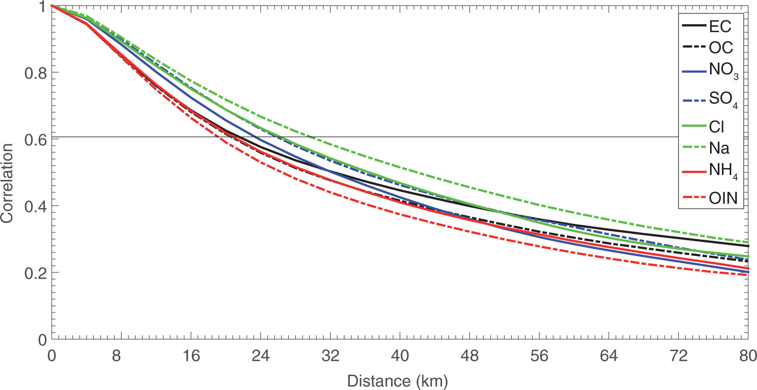
Fig. 5
Horizontal correlation curves of the background errors for each species. The blue line denotes the length scale at the position of .
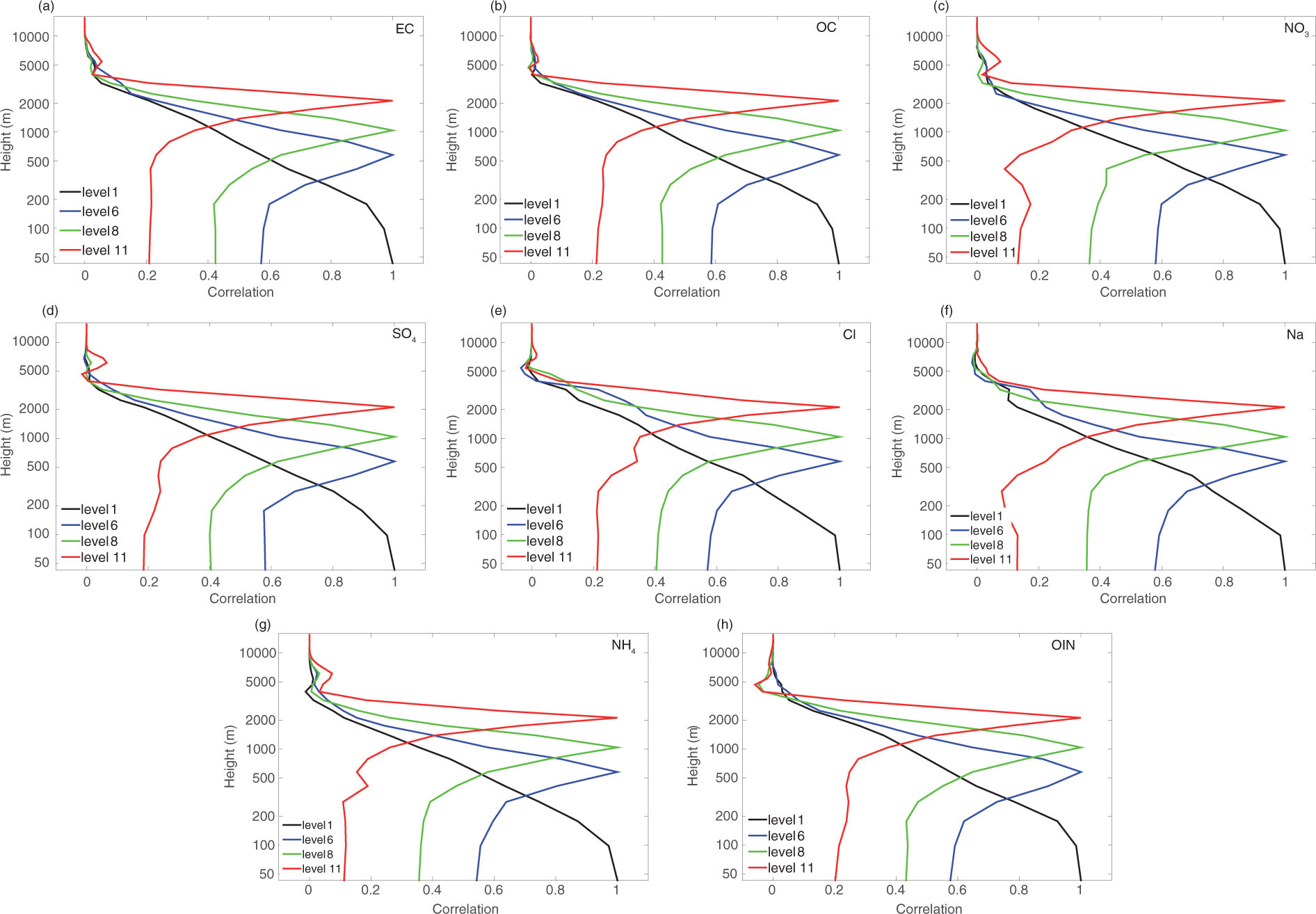
Fig. 6
Profiles of vertical correlation of the background error for EC (a), OC (b), NO3 (c), SO4, (d), Cl (e), Na (f), NH4 (g) and OIN (h). One curve represents the correlation of a given level with all the levels. The given levels include the surface and other three levels.
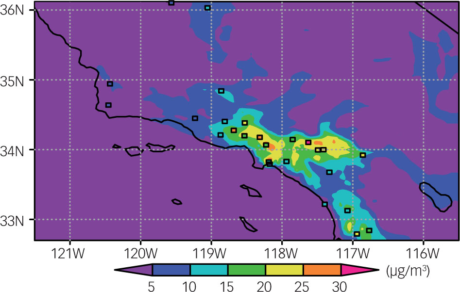
Fig. 7
Background (shaded) and surface observations (squares) of PM2.5 at 02:00 PDT 2 June 2010. The colour differences between the shaded areas and squares indicate the innovations of the surface PM2.5 concentration observations.
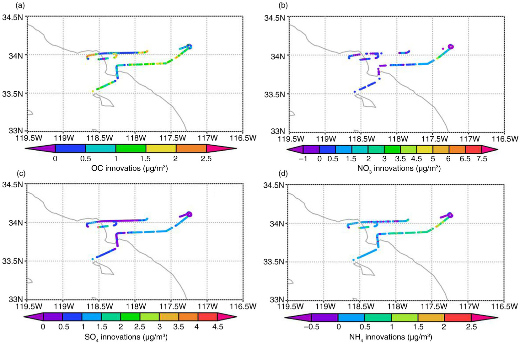
Fig. 8
Observation innovations of species of OC (a), NO3 (b), SO4 (c), and NH4 (d) along the aircraft flight track between 01:30 and 02:30 PDT 2 June 2010.
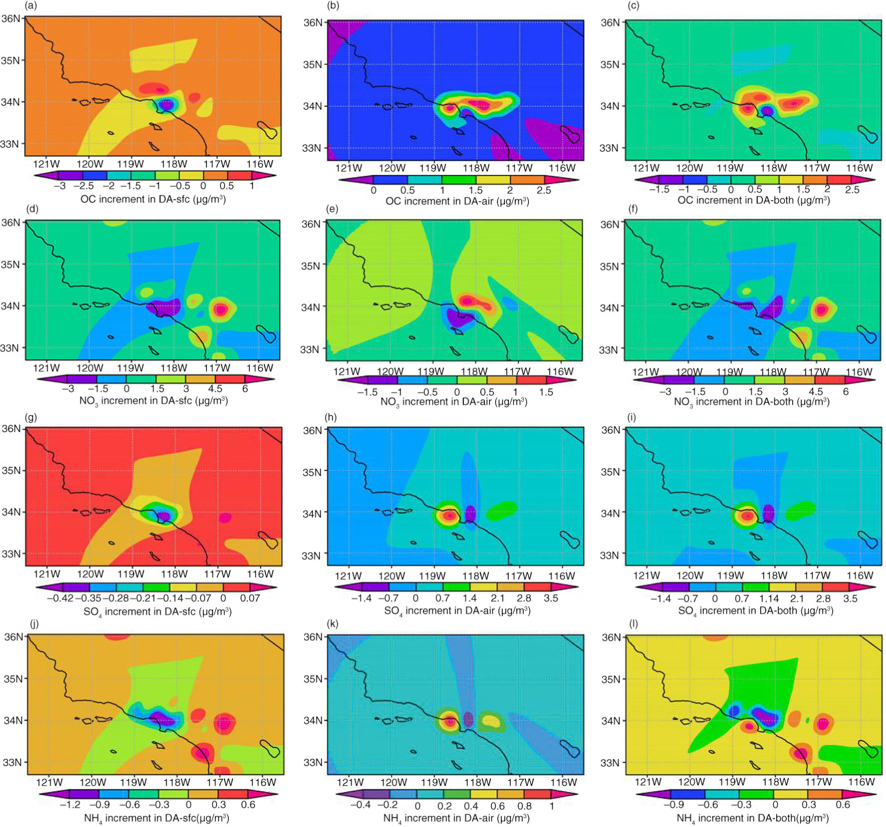
Fig. 9
Surface distributions of increments of the species in three DA experiments. Each column contains the increments from the same DA experiment. Figures in the left, middle and right columns are from DA-sfc, DA-air and DA-both, respectively. Figures in each row are from the species of OC (a, b, and c), NO3 (d, e and f), SO4 (g, h and i) and NH4 (j, k and l) from top to bottom, respectively.
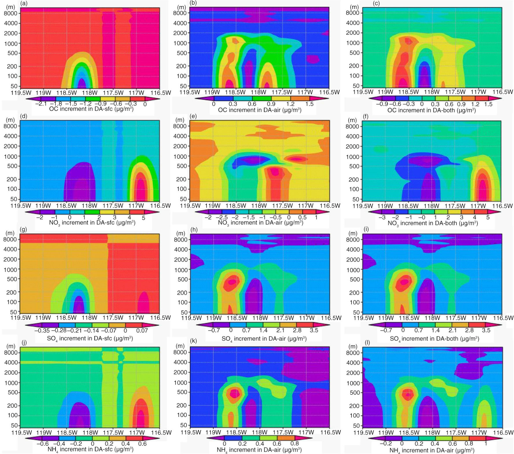
Fig. 10
Same as Fig. 9 except for vertical sections along 33.80N.
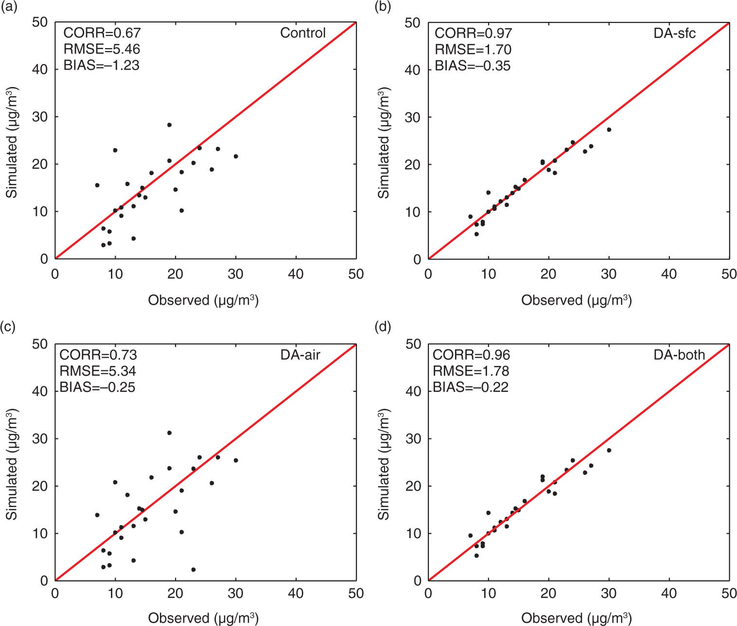
Fig. 11
Scatter plots of observed concentrations of PM2.5 versus simulated concentrations of PM2.5 from the experiments of Control (a), DA-sfc (b), DA-air (c) and DA-both (d) surface over 02:00 PDT initialisations. The observed concentrations of PM2.5 are from the 42 surface stations, and they are used in the assimilation of DA-sfc and DA-both.
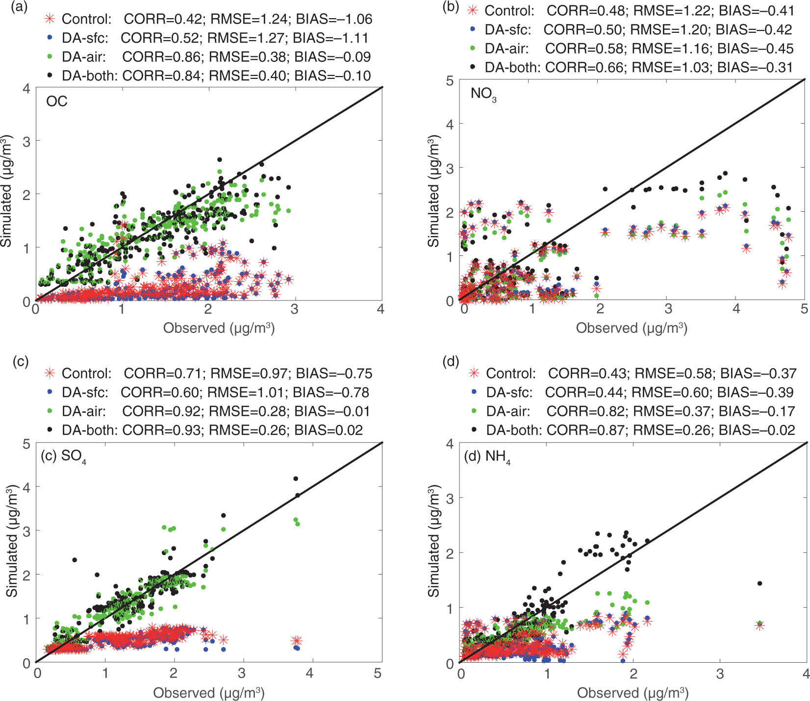
Fig. 12
Scatter plots of observed concentrations of OC (a), NO3 (b), SO4 (c) and NH4 (d) versus simulated concentrations during 01:30 to 02:30 PDT initialisations. The CORR, RMSE and BIAS are estimated for all the four experiments: Control (red start), DA-sfc (blue dot), DA-air (green dot) and DA-both (black dot). The observed concentrations of species are from the aircraft observations, and they are used in the assimilation of DA-air and DA-both.
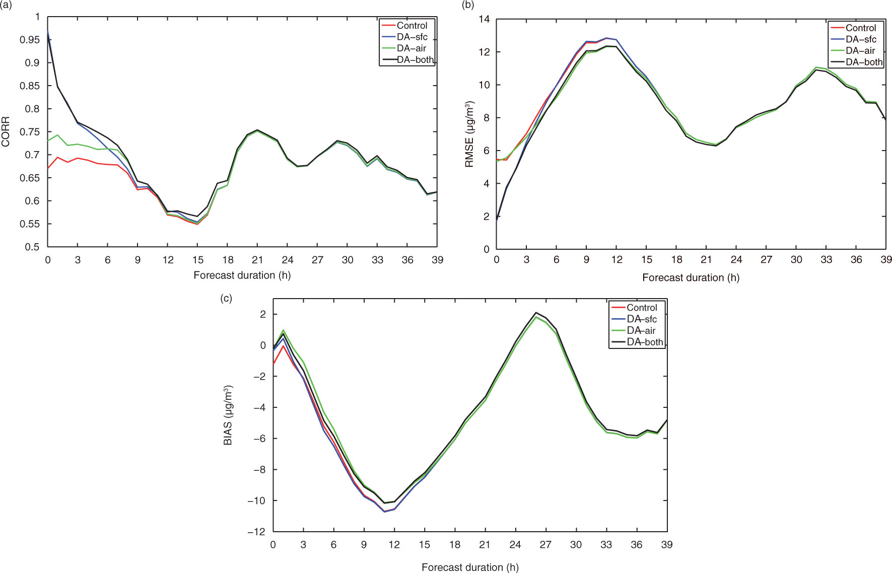
Fig. 13
Correlations (CORR) (a), root-mean-square errors (RMSE) (b) and BIAS (c) of the total PM2.5 concentration forecasts against observations as a function of forecast duration. All of them are calculated against the observations from 42 surface stations during the period from 02:00 PDT 2 June to 17:00 PDT 3 June 2010.
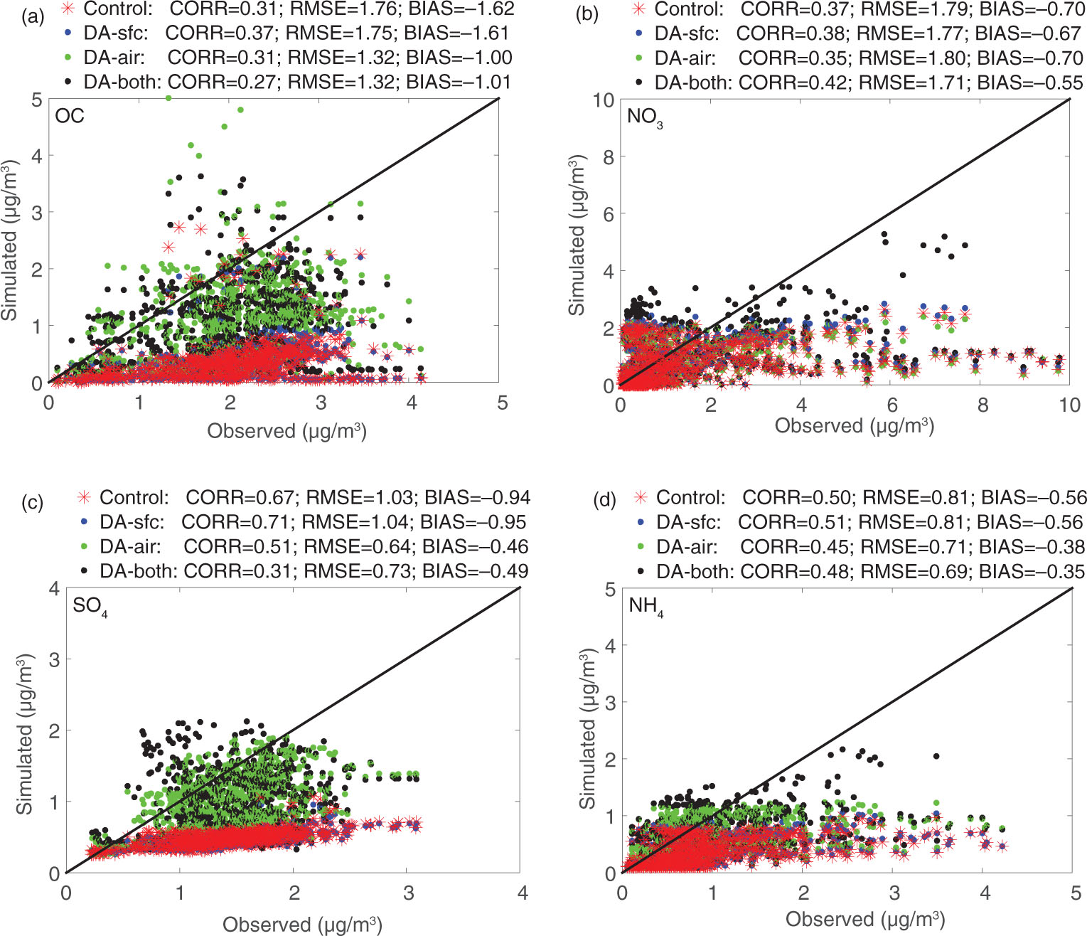
Fig. 14
Same as Fig. 12 except for the observed concentrations versus forecast concentrations during 02:30–07:00 PDT 2 June.