
Table 1. MsTMIP models and simulations used in this study
ModelSG1SG2SG3BG1References
BIOME-BGCOO Thornton et al. (2002)CLASS-CTEM-NaOOOO Huang et al. (2011) CLM4OOOO Shi et al. (2011), Mao et al. (2012) CLM4VICOOOO Lei et al. (2014) DLEMOOOOTian et al. (2011, 2012)GTECOOO Ricciuto et al. (2011) ISAMOOOO Jain and Yang (2005)LPJ-wslOOO Sitch et al. (2003)ORCHIDEE-LSCEOOO Krinner et al. (2005)SiB3-JPLOOO Baker et al. (2008)SiB3CASAOOO Schaefer et al. (2008)TEM6OOOO Hayes et al. (2011) TRIPLEX-GHGOOO Zhu et al. (2014) VEGAS2.1OOO Zeng et al. (2005)VISITOOO Ito and Inatomi (2012)
[iii] Biome-BGC, Global Biome Model-Biogeochemical Cycle; MsTMIP Multi-scale Terrestrial Model Intercomparison Project (MsTMIP); CLASS-CTEM-N, Canadian Land Surface Scheme and Canadian Terrestrial Ecosystem Model with Nitrogen; CLM4, Community Land Model version 4; CLM4VIC, Community Land Model version 4 with Variable Infiltration Capacity Runoff Paramaterization; DLEM, Dynamic Land Ecosystem Model; GTEC, Global Terrestrial Ecosystem Carbon model; ISAM, Integrated Science Assessment Model; LPJ-wsl, Lund-Potsdam-June model by Swiss Federal Institute for Forest, Snow, and Landscape Research; ORCHIDEE-LSCE, Organising Carbon and Hydrology in Dynamic Ecosystems; SiB3-JPL: Simple Biosphere version 3 by Jet Propulsion Laboratory; SiBCASA, Simple Biosphere with Carnegie-Ames-Stanford Approach; TEM6, Terrestrial Ecosystem Model version 6; TRIPLEX-GHG, a process-based GHG model developed from three models; VEGAS2.1, Vegetation Global Atmosphere and Soil version 2.1; VISIT, Vegetation Integrative SImulator for Trace gases.
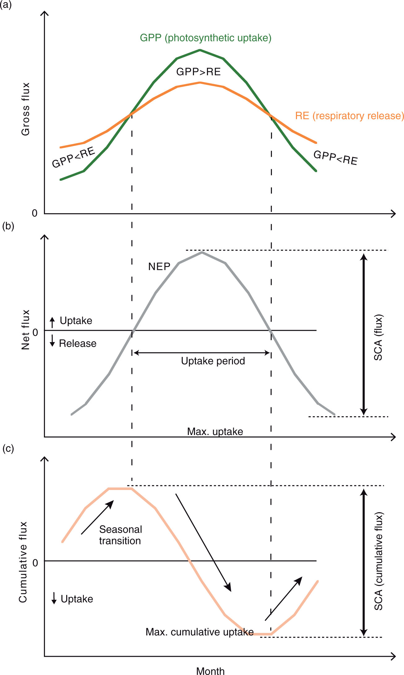
Fig. 1
Explanation of seasonal-cycle amplitude (SCA) metrics with idealized sample data. (a) Seasonal change in gross CO2 fluxes: GPP, gross primary production, and RE, ecosystem respiration. (b) Seasonal change in net CO2 flux (NEP, net ecosystem production) and its seasonal amplitude. (c) Seasonal change in cumulative CO2 flux in calendar year and its SCA.
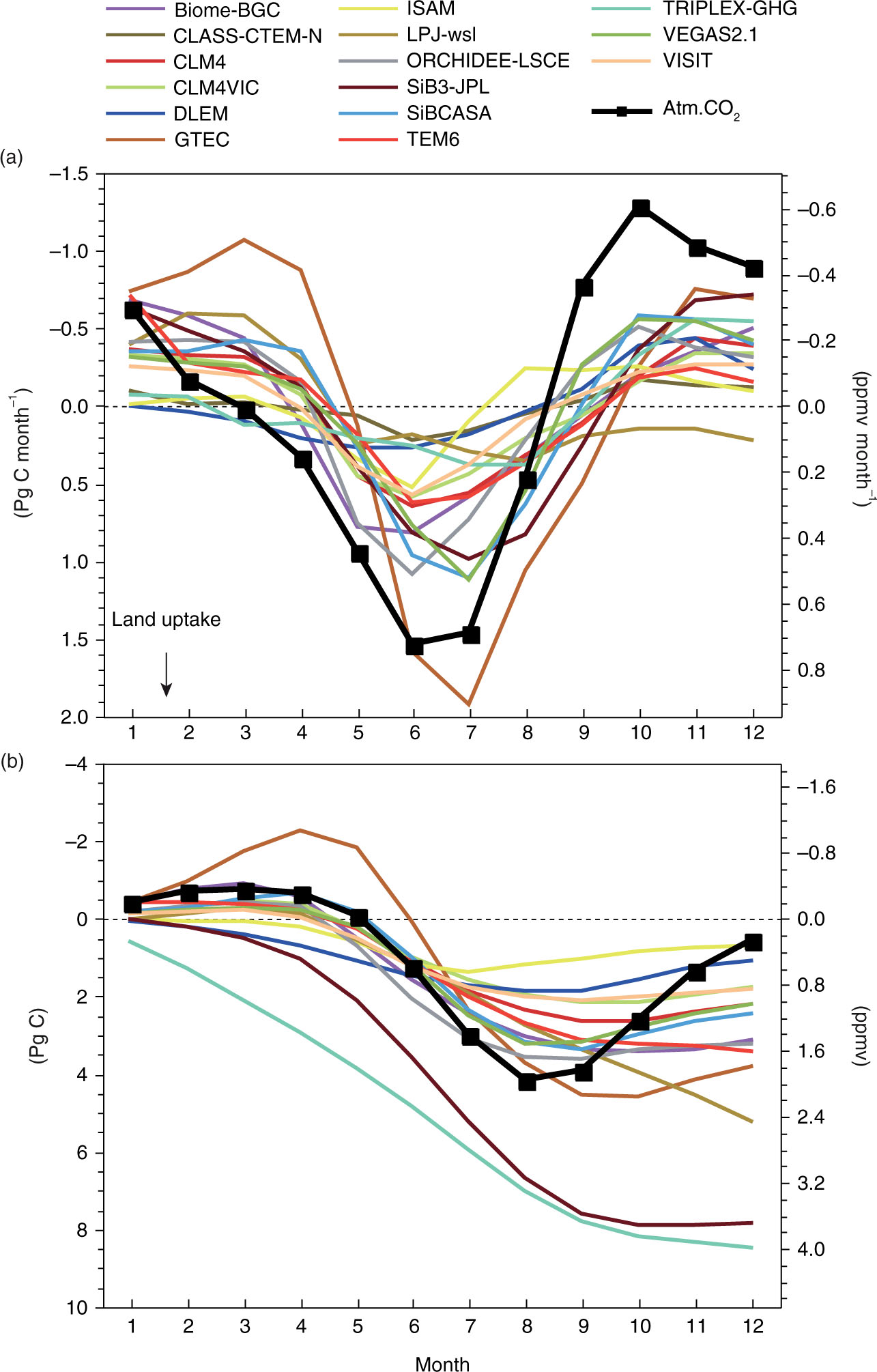
Fig. 2
Average seasonality of net ecosystem production estimated by 15 MsTMIP models and atmospheric CO2 concentration. Global-mean atmospheric CO2 data from 1984 to 2010 were obtained from the World Data Center for Greenhouse Gases (URL: http://ds.data.jma.go.jp/gmd/wdcgg/wdcgg.html). Model results of SG3 or BG1 (if available) for the same period were used. (a) Monthly net ecosystem production (positive for net sink) compared to monthly atmospheric CO2 concentration change [i.e. Δ(CO2)/Δt]. For both terrestrial fluxes and atmospheric CO2, anomalies from the annual mean values are shown. (b) Cumulative net ecosystem production compared with seasonal changes in atmospheric CO2 concentrations.
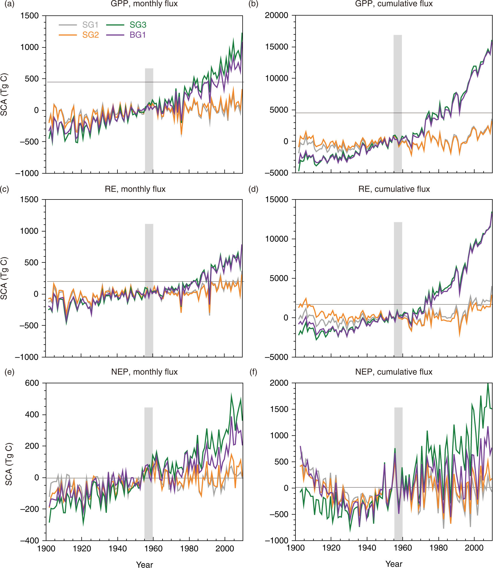
Fig. 3
Interannual variability of the SCA of global terrestrial CO2 fluxes. For each of the simulations (SG1, SG2, SG3 and BG1), model-average anomalies of the MsTMIP models against the 1950s-mean (grey zone) are shown. (a) Monthly GPP, (b) cumulative (i.e. annual total) GPP, (c) monthly RE, (d) cumulative RE, (e) monthly NEP and (f) cumulative NEP.
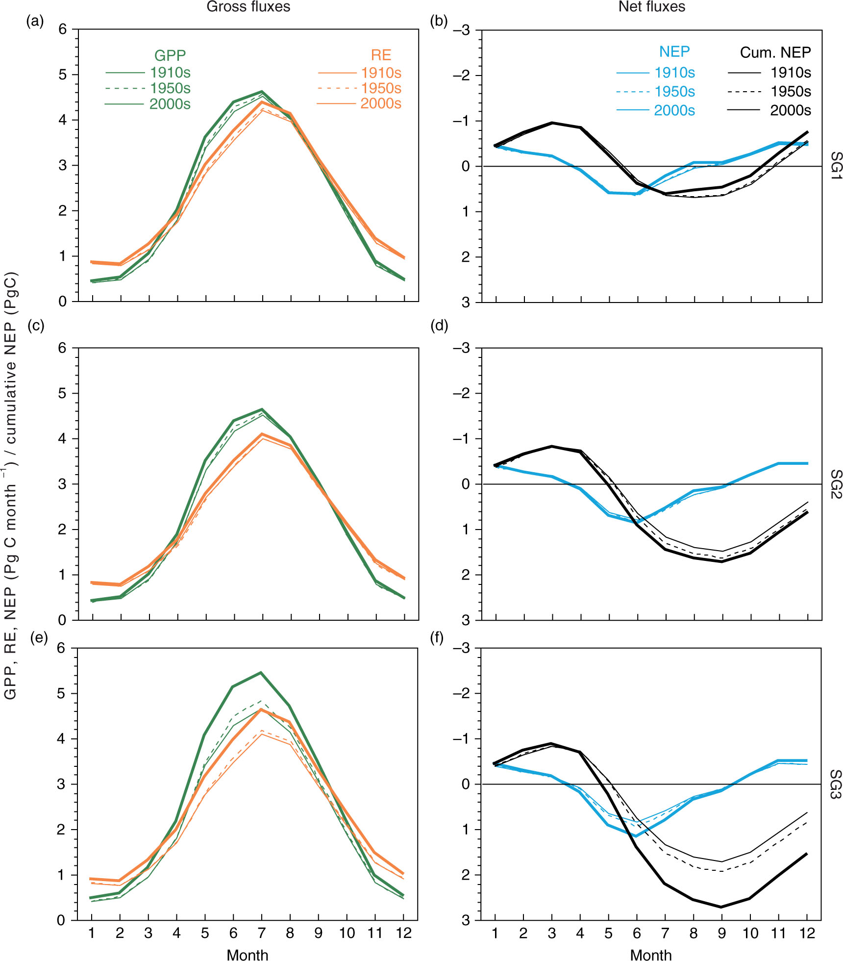
Fig. 4
Mean seasonal-cycle of gross and net CO2 fluxes in the northern middle latitudinal zone (25–55°N) for different periods: the 1910s, 1950s and 2000s. Averages of MsTMIP model results for (a, b) SG1, (c, d) SG2 and (e, f) SG3 simulations.
Table 2. Simulated linear trends in the seasonal-cycle amplitude (SCA) of global terrestrial CO2 fluxes
ExperimentGPPRENEPCum. NEP
SG1+0.023+0.068−0.011−0.024SG2+0.042+0.062+0.014+0.064SG3+0.257+0.222+0.276+0.496BG1+0.209+0.209+0.190+0.382Atmospheric CO2 trends
Global mean (1984–2010)a+0.29
Barrow (1961–2011)b+0.60
Mauna Loa (1958–2011)b+0.32
[i] Averages of MsTMIP models are shown. For comparison, linear trends in seasonal amplitude of atmospheric CO2 concentration are also shown (see text).
[ii] aSee Supplementary Fig. 1.
[iii] bFrom Graven et al. (2013).
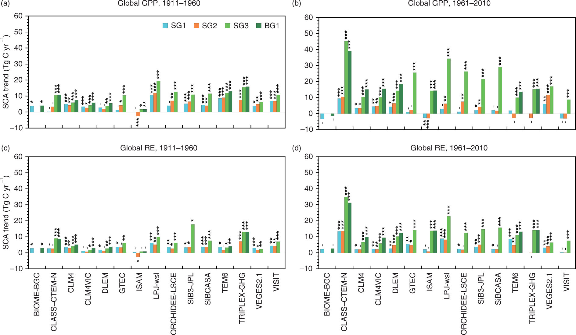
Fig. 5
Linear trends in the SCA of gross fluxes simulated by the MsTMIP models in different periods. (a, b) GPP and (c, d) RE for (a, c) 1911–1960 and (b, d) 1961–2010: ***, p<0.001; **, p<0.01; *, p<0.05; –, insignificant.
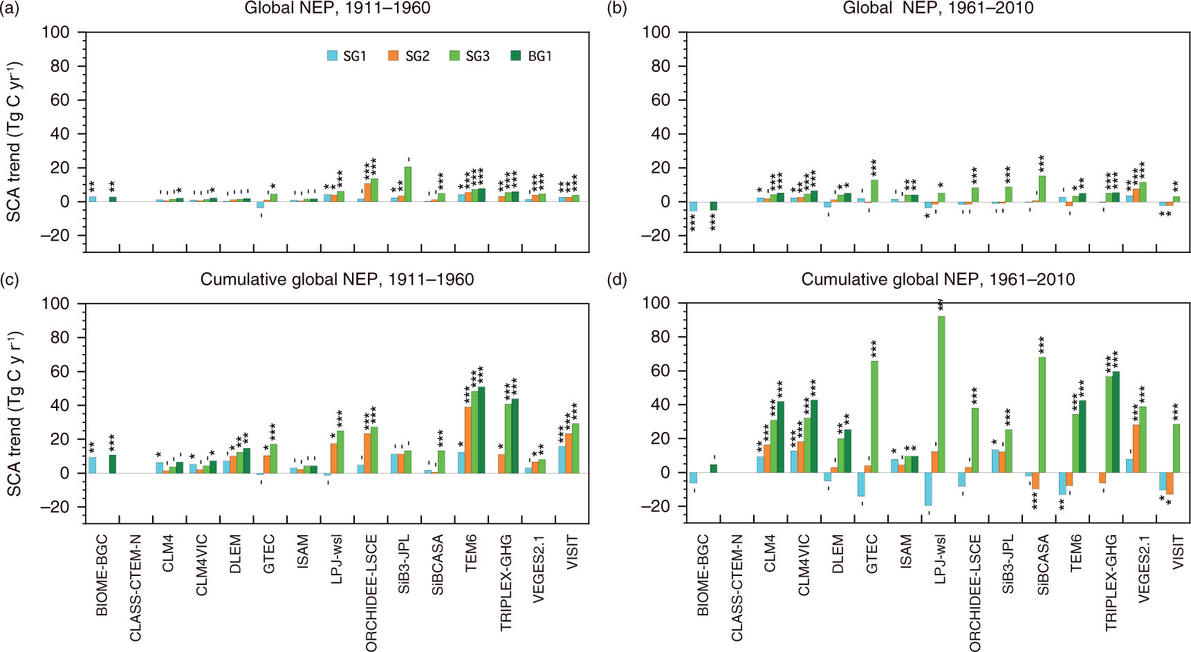
Fig. 6
Linear trends in the SCA of net fluxes simulated by the MsTMIP models in different periods. (a, b) Monthly NEP and (c, d) cumulative NEP for (a, c) 1911–1960 and (b, d) 1961–2010: ***, p<0.001; **, p<0.01; *, p<0.05; –, insignificant. Result of CLASS-CTEM-N is not shown here, because NEP (= GPP − RE) was always negative.
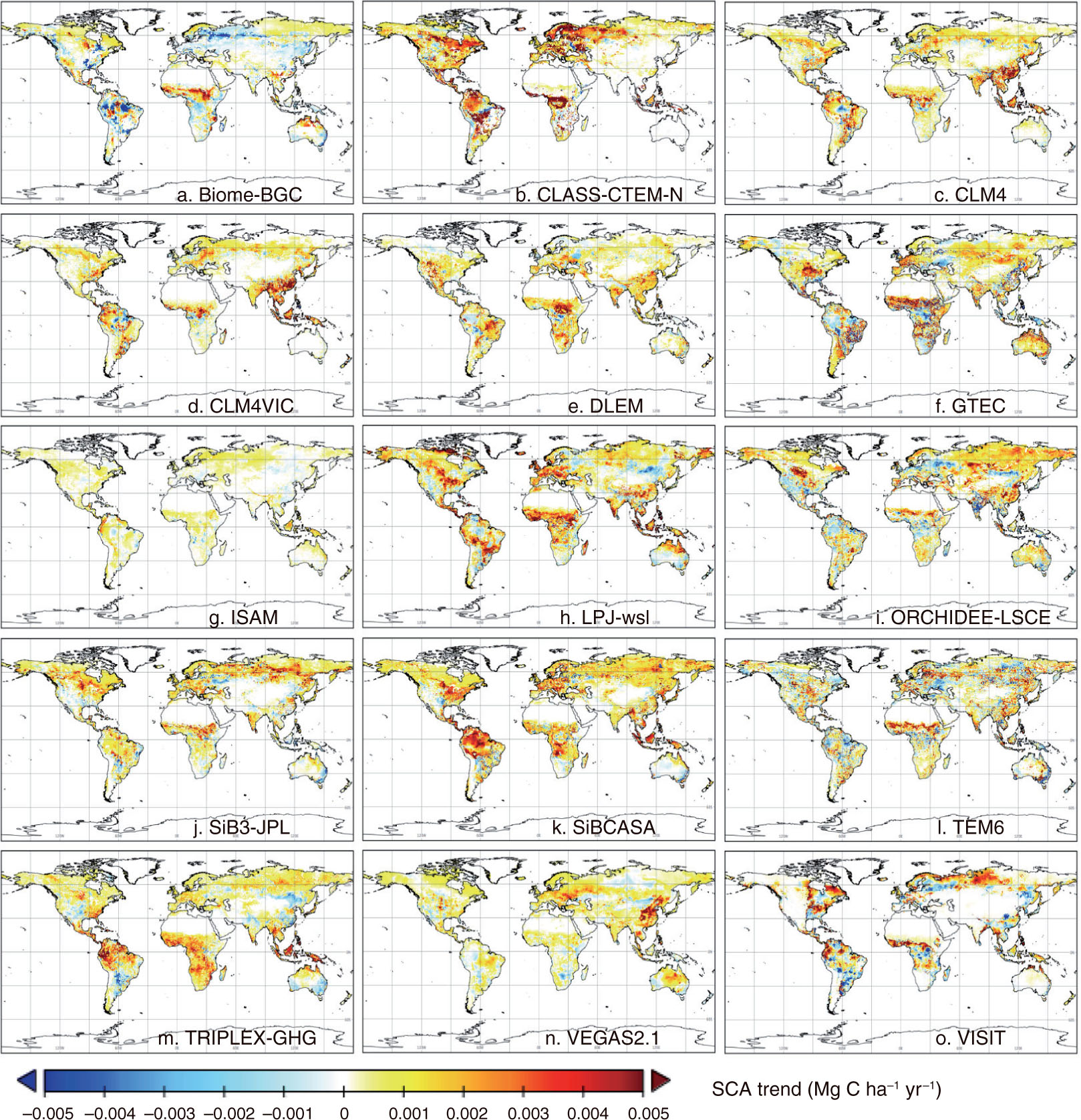
Fig. 7
Distribution of linear trends of the SCA of the cumulative NEP estimated by 15 MsTMIP models during the period 1982–2010 (i.e. comparable to data used in Fig. 10a).
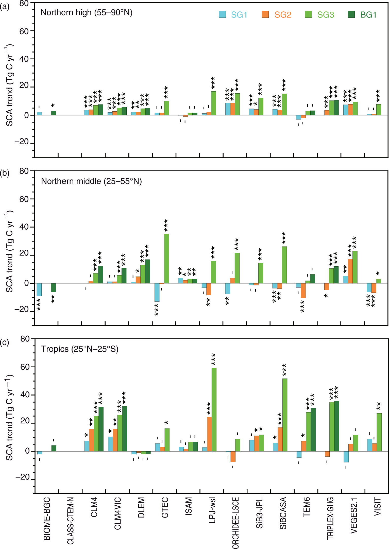
Fig. 8
Linear trends of the SCA of cumulative NEP estimated by MsTMIP models in 1961–2010 for different latitudinal zones. (a) Northern high (55–90°N), northern middle (25–55°N) and tropics (25°N–25°S): ***, p<0.001; **, p<0.01; *, p<0.05; –, insignificant.
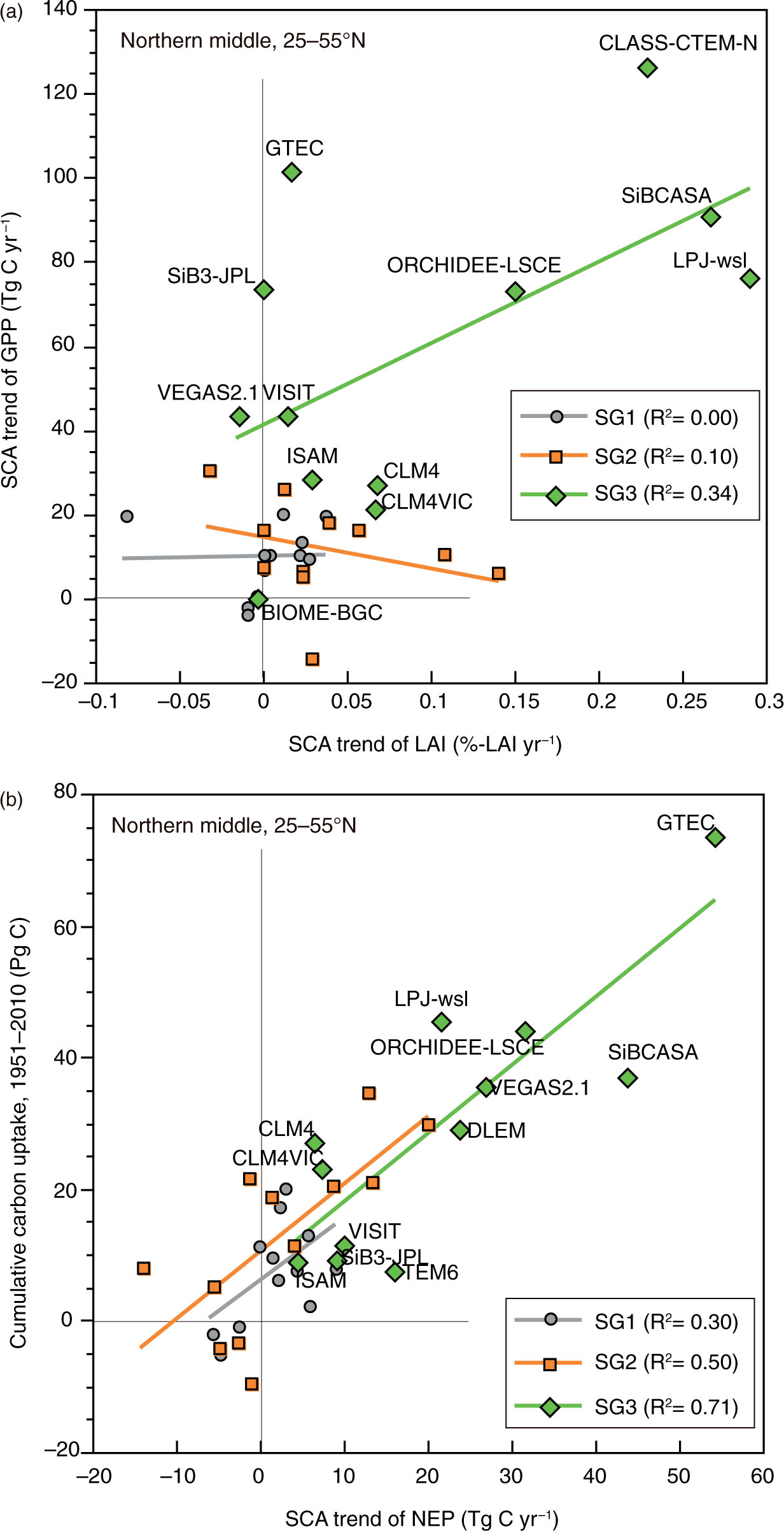
Fig. 9
Relationship between the SCA metrics and carbon budget metrics. Results of the northern middle latitude (25–55°N) in 1961–2010 for SG1, SG2 and SG3 simulations are shown. (a) Relationship between the trend of the SCA of leaf area index (LAI, model estimation) and the trend of the SCA of monthly GPP. (b) Relationship between the trend of the SCA of cumulative NEP and accumulated carbon uptake during the period.
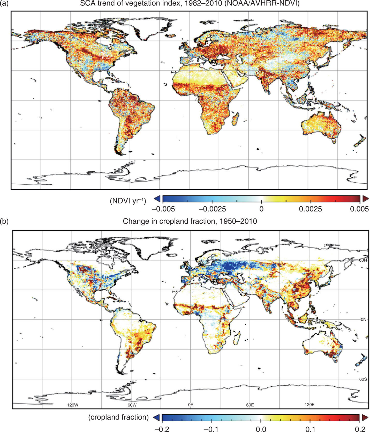
Fig. 10
(a) Distribution of the linear trend of the SCA (i.e. max–min difference) of the Normalized Difference Vegetation Index (NDVI) in 1982–2010, and (b) distribution of the change in cropland fraction 1950–2010 obtained from the data set by Hurtt et al. (2011).