
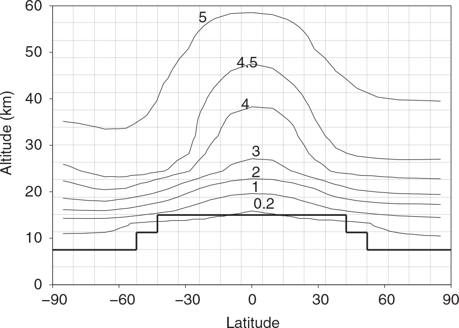
Fig. 1
Simulated time spent by an air mass in the stratosphere, in years (‘age of stratospheric air’). The thin dashed line is the model grid; the thick line is the model tropopause. Note that the crossing of the tropopause by the 0.2 yr isoline is due to interpolating on the too coarse grid.
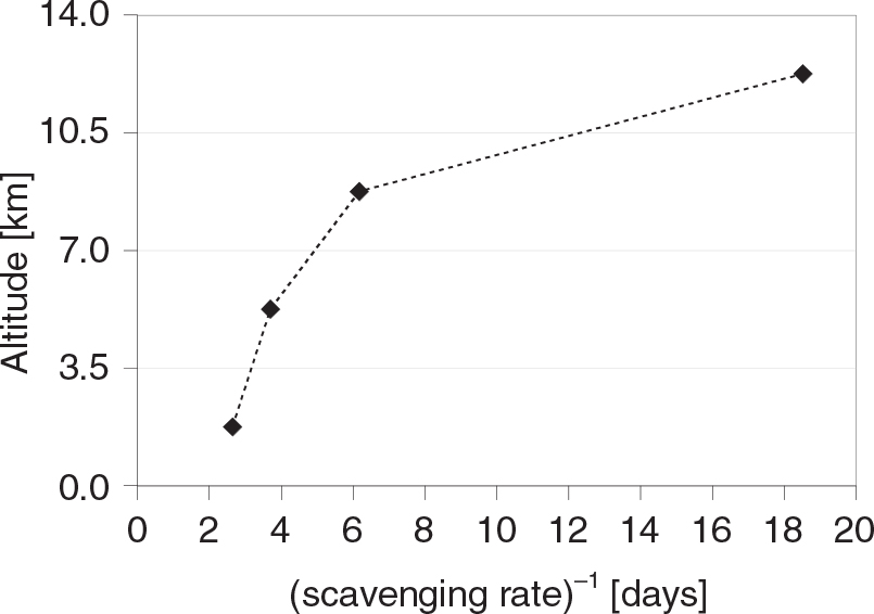
Fig. 2
Scavenging rates applied to particles and beryllium atoms in the model troposphere.
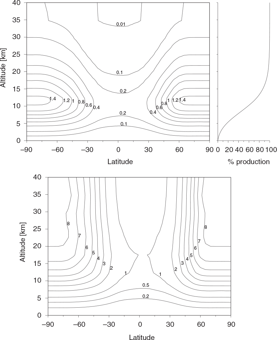
Fig. 3
Production rate of Be-10 for Φ = 600 MV. Altitudes are approximate. Top: production rate independent of air expressed in atoms per year per actual cubic centimetre. Cumulated profile on the right. Bottom: production rate dependent of air, expressed in atoms per year per standard cubic centimetre.
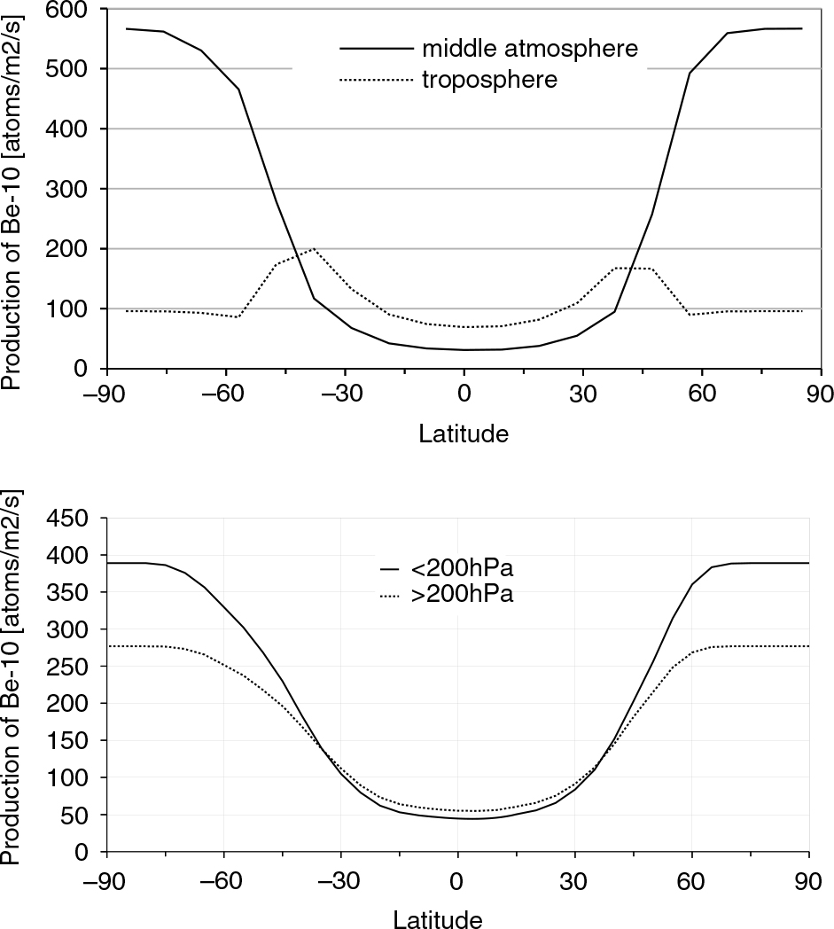
Fig. 4
Vertically integrated production rate of Be-10 through the middle and lower parts of the atmosphere to sea level. (Top) Vertical definition based on our model definition of the tropopause, and (bottom) definition based on pressure.
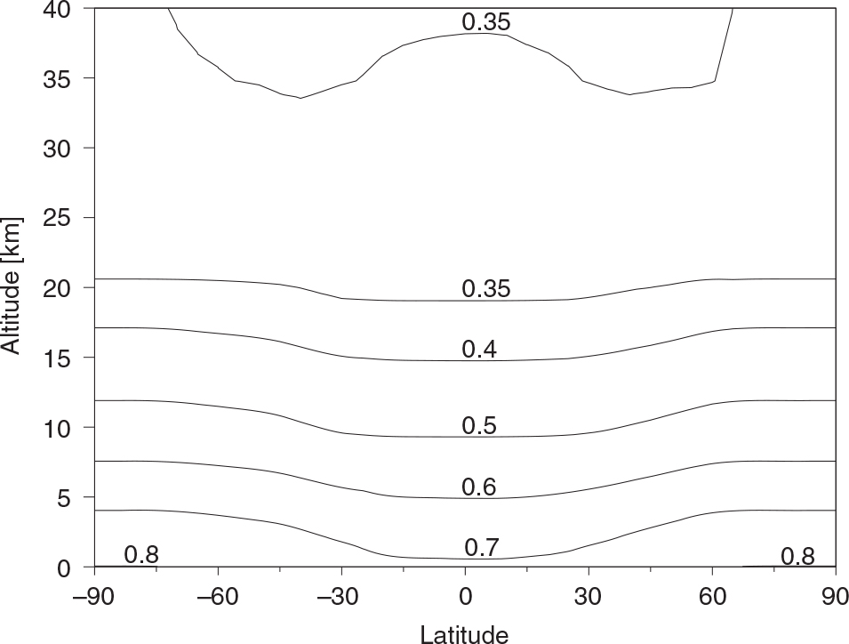
Fig. 5
Ratio of Be-10 to Be-7 production rates.
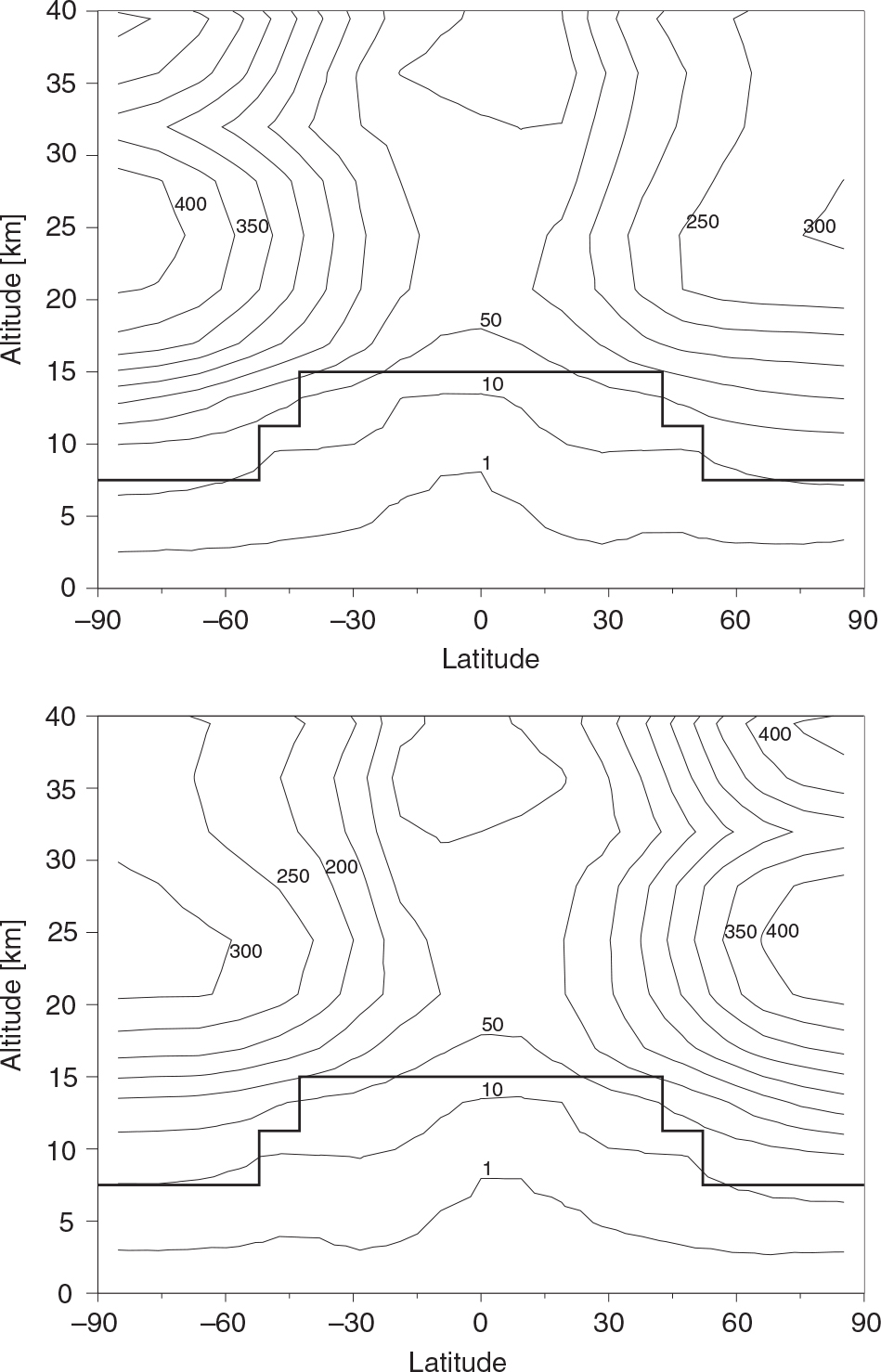
Fig. 6
Simulated concentration of Be-7 in the atmosphere, in 104 atoms per standard cubic meter (SCM), for January (top) and July (bottom). The thick line represents the tropopause in the model.
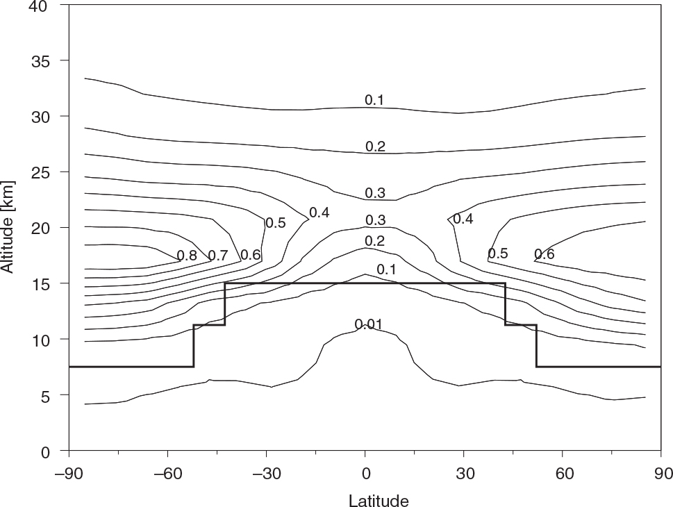
Fig. 7
Simulated annual concentration of Be-10, in atoms per (real) cubic centimetre. The thick line represents the tropopause in the model.
Table 1. Key figures about Be-10 and Be-7 determined in this study (note that ‘middle atmosphere’ stands for the model domain above the tropopause)
62%3.3×10¹⁷
68%1.5×10¹⁷
62%3.3×10¹⁷
68%Atmospheric burden (atoms) and middle atmosphere proportion2.8×1024
96%1.2×1024
91%5.5×1024
98%1.2×1024
92%Middle atmosphere residence time with respect to production (months)11.41.822.71.8Tropospheric residence time (days)9 wrt. total production11 wrt. tropospheric production9 wrt. total production11 wrt. tropospheric production
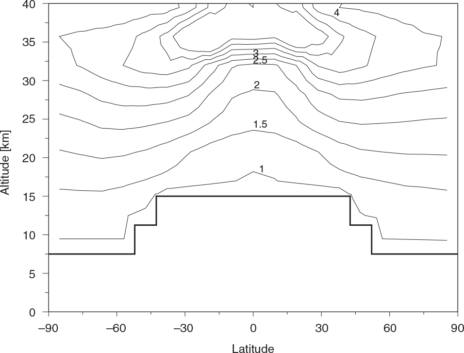
Fig. 8
Ratio of Be-10 concentrations simulated without and with sedimentation of particles.
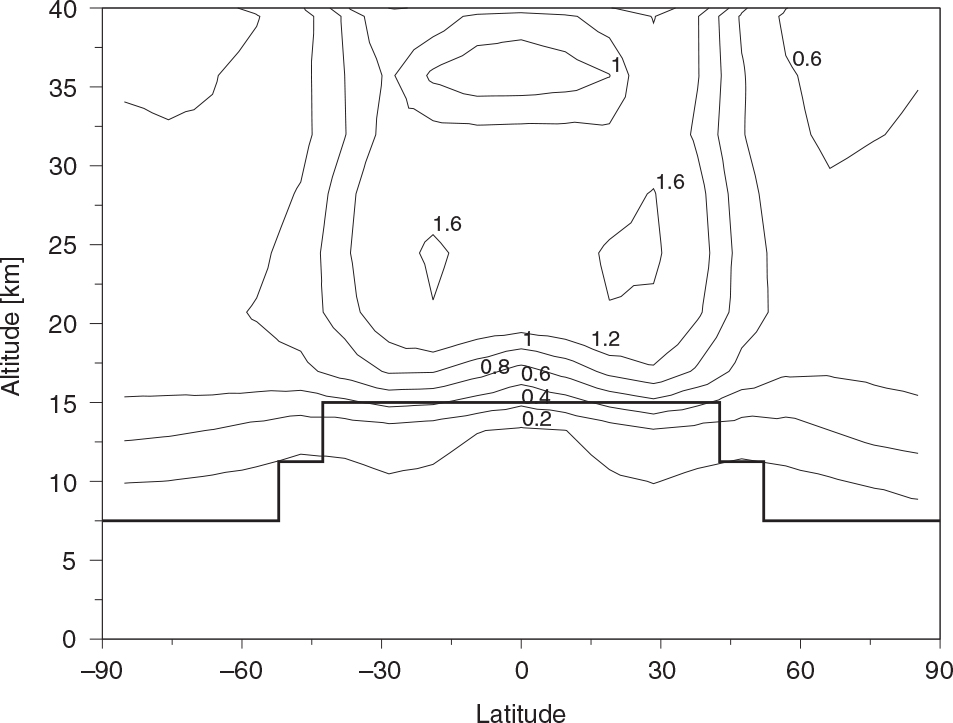
Fig. 9
Ratio of simulated Be-7 concentration to the calculated Be-7 concentration at ‘secular equilibrium’ (balance between production and radioactive decay), also called ‘saturation ratio’.
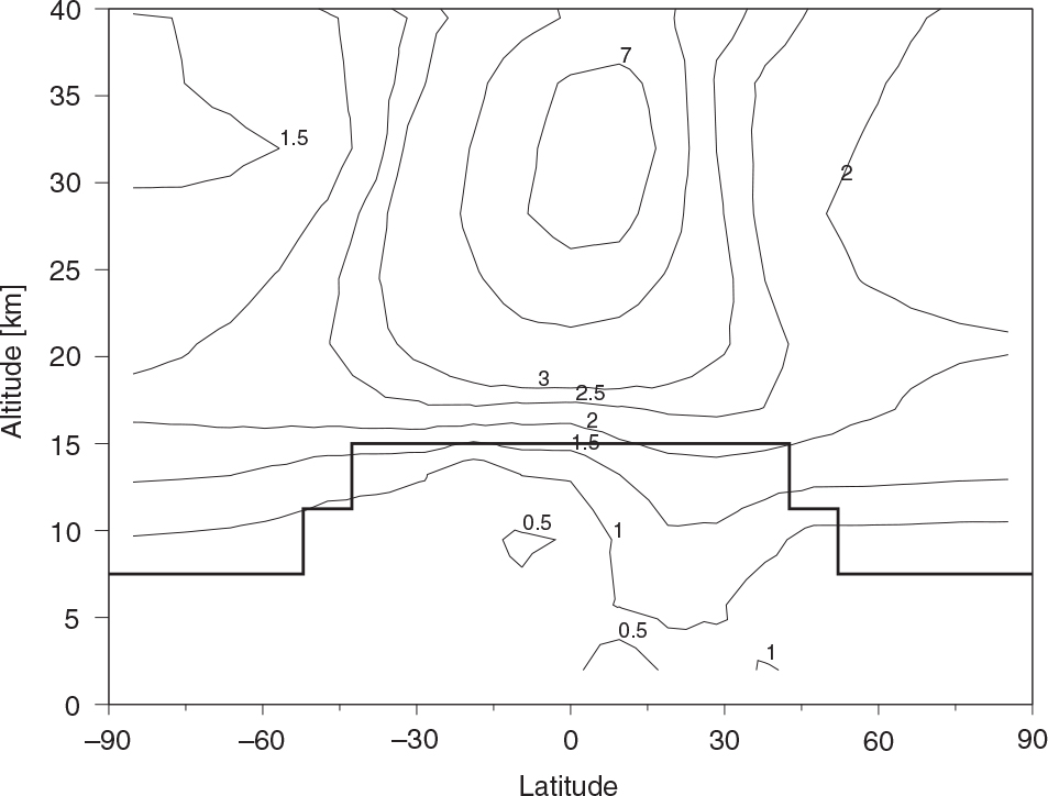
Fig. 10
Ratio of simulated Be-10 to Be-7 concentrations for January.
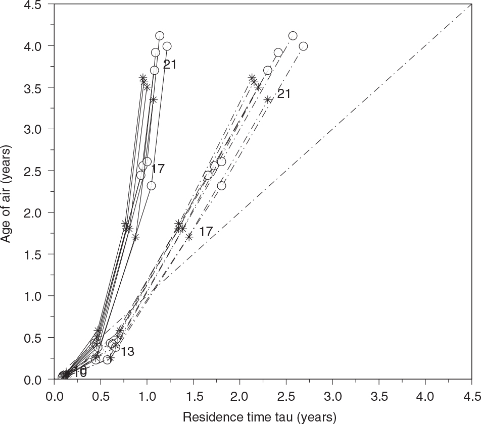
Fig. 11
Simulated vertical profiles of age of air vs. residence time τ of aerosols. Four levels are represented, at approximately 10, 13, 17 and 21 km (cf. labels). Full lines: simulation with beryllium sedimentation; dashed–dotted lines: simulation without sedimentation. Circles underline southern high-latitude profiles (approx. 85°S to 57°S); stars underline northern high-latitude profiles (approx. 85°N to 57°N).