
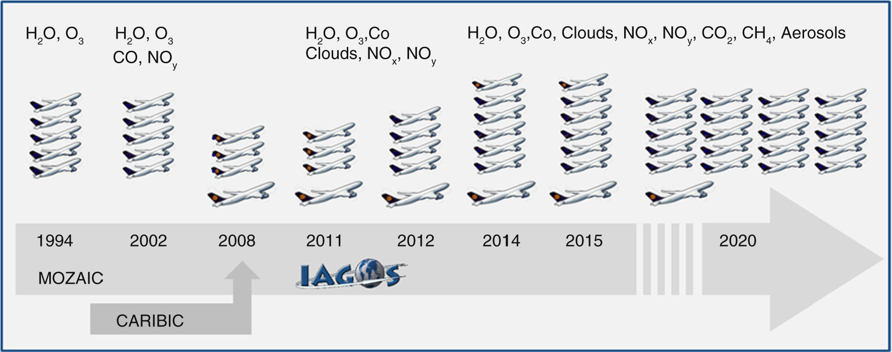
Fig. 1
Evolution of airborne observations using instrumented passenger aircraft from programmes MOZAIC and CARIBIC to IAGOS: the aircraft represent the number of equipped units in operation, with the larger aircraft symbol representing IAGOS-CARIBIC. Observation parameters are indicated for the various evolution stages of the programme.
Table 1. Objectives and scientific value of IAGOS research infrastructure
Open data policy (GEO/GEOSS)IAGOS-COREAtmosphere monitoring by up to 20 long-haul aircraft equipped with scientific instruments for
• atmospheric chemical composition
• (H2O, O3, CO, NO x , NO y , CO2, CH4)
• aerosol particles
• cloud particles
Global-scale coverage of observations
Near real-time data provision for CAMSIAGOS-CARIBICMonthly deployment of the instrumented CARIBIC container aboard one aircraft
Measurement of a large number of species (~100), including those of IAGOS-CORE plus
• stratospheric H2O, cloud ice/water
• N2O, SF6, VOCs
• (H)CFCs
• NMHCs
• aerosol particle elemental composition
• H2O isotopologues and
• HgScientific valueChanges in the tropopause regionHigh spatial and temporal resolution of in-situ observations
Ozone background and trend
Water vapour background and trend
Stratosphere–troposphere exchange and related transport mechanismsValidation of atmospheric models and satellite retrievalsTropospheric profiles of H2O, O3, CO, NO x , CO2, CH4, aerosols, cloud particles
UTLS data of H2O, O3, CO, NO x , CO2, CH4, aerosols, cloud particlesGlobal air qualityInfluence of developing regions
Long-range transport of air pollutants
Vertical transport of air pollutants by deep convectionInternational transfer standardsUse of proven measurement technology
Global deployment of identical instruments
Regular quality assurance including calibration against reference instruments, based on GAW standard procedures
Table 2. Current IAGOS fleet
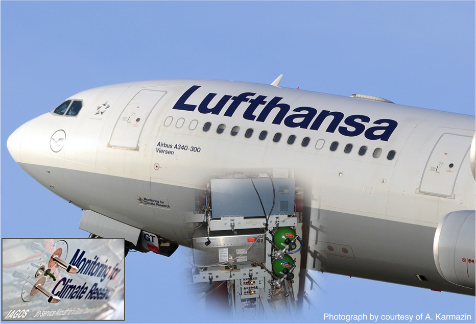
Fig. 2
IAGOS-CORE installation position aboard the Lufthansa A340-300 ‘Viersen’ (photograph by courtesy of A. Karmazin); the inset shows details of the IAGOS Inlet Plate, which carries the inlet probes for trace gas sampling (photograph by courtesy of Lufthansa).
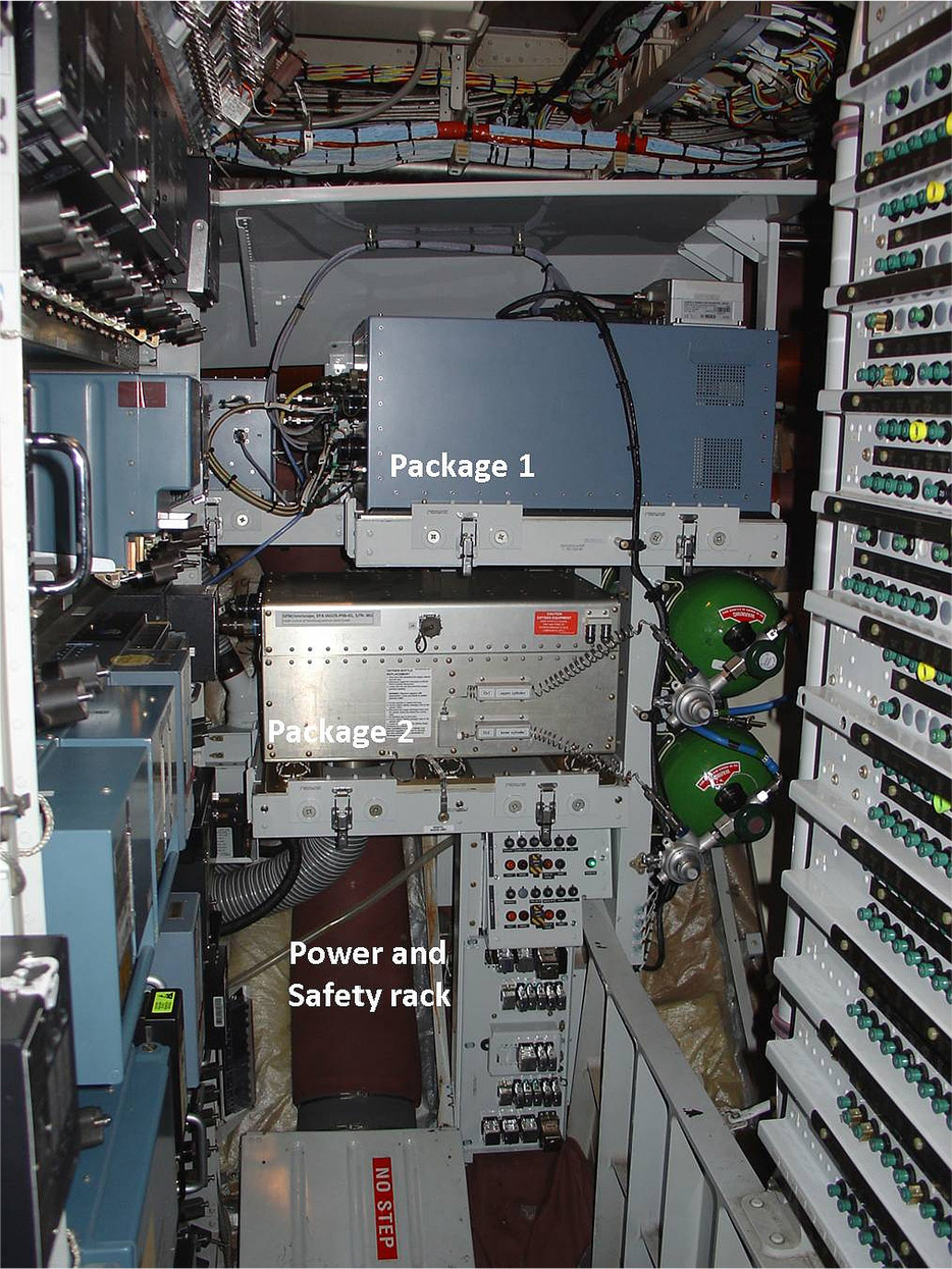
Fig. 3
Installation of IAGOS-CORE instrumentation in the avionics bay of Lufthansa D-AIGT.
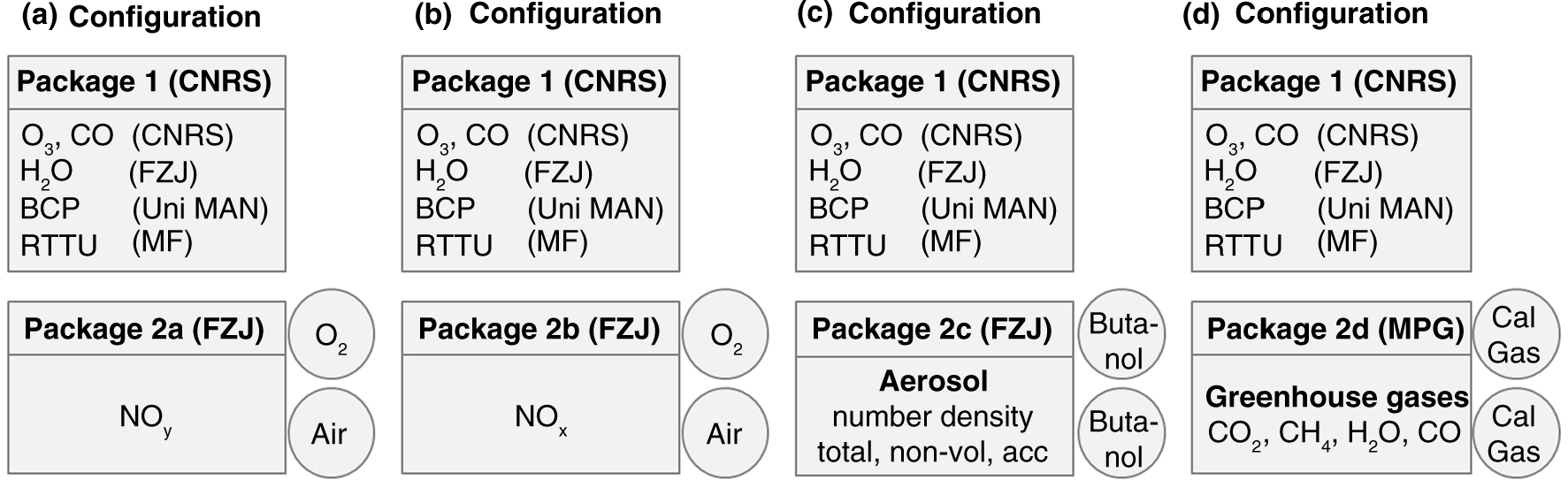
Fig. 4
Available configurations for IAGOS-CORE instrumentation.
Table 3. IAGOS-CORE instrumentation
Optical particle counter (0.25–3 µm)4 s±10 cm−3
±5 cm−3FZJ/DLR (Bundke et al., 2015)Opt. dCO2
CH4
H2O
COCavity ring-down spectroscopy4 s±0.1 ppm
±2 ppb
±6–15 ppm
±10 ppbMPI-BGC (Filges et al., 2015)
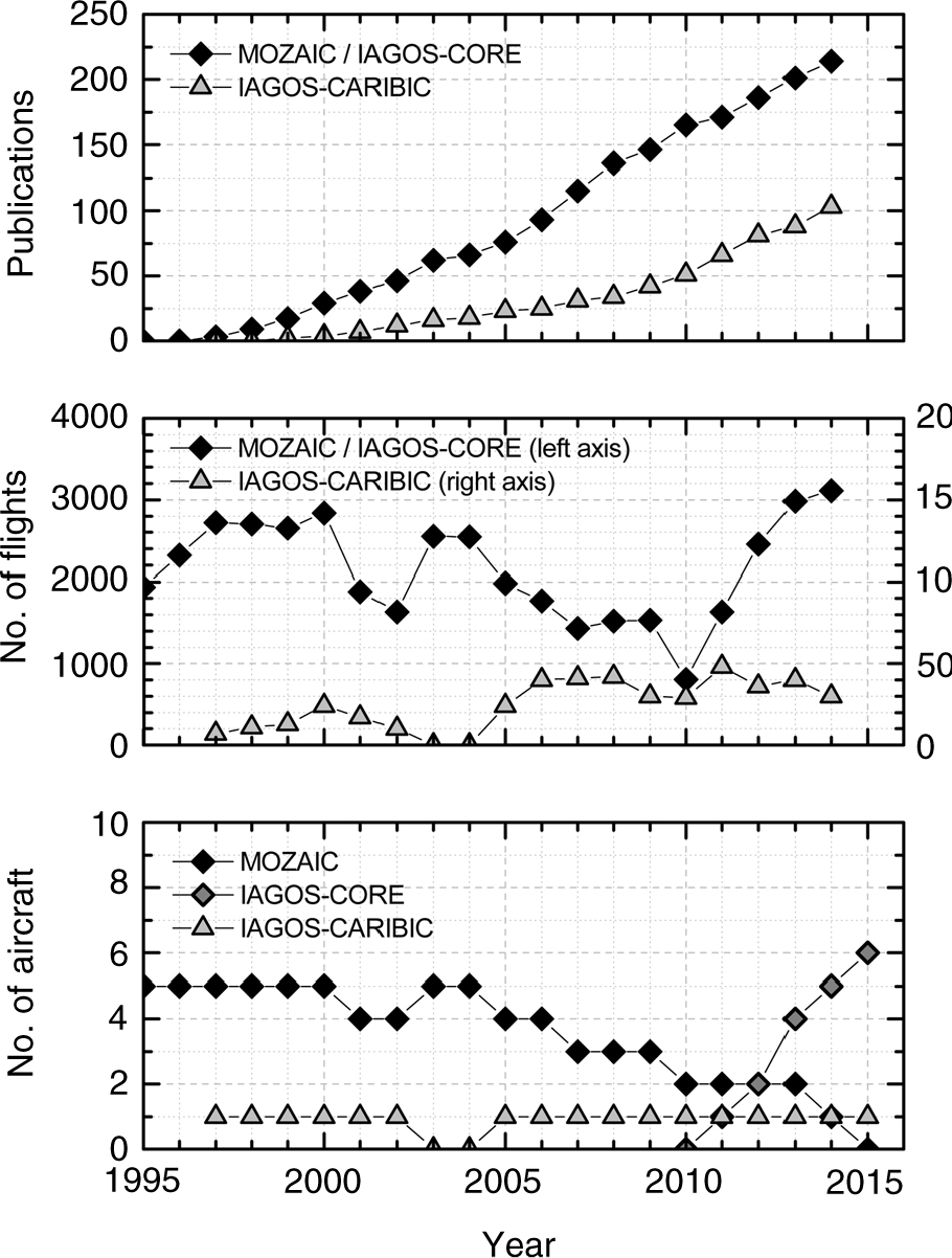
Fig. 5
Number of aircraft in operation (bottom panel), number of flights (mid-panel) and cumulative number of scientific publications (top panel) for MOZAIC (until 2014), IAGOS-CORE (from 2011) and IAGOS-CARIBIC.
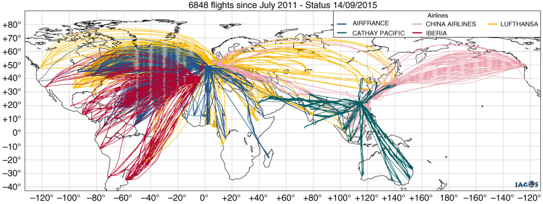
Fig. 6
Map of IAGOS-CORE flights from July 2011 to August 2015.
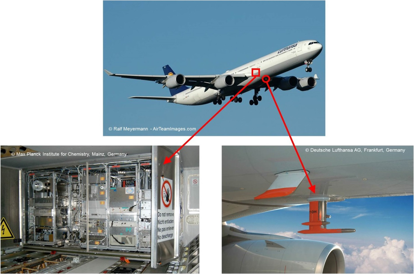
Fig. 7
IAGOS-CARIBIC aircraft, air inlet system and measurement container (Brenninkmeijer et al., 2007).
Table 4. IAGOS-CARIBIC instrumentation (as of 2015)
Chemiluminescence4 s
0.2 s±0.5 ppbv or 1% (the higher)KIT (Zahn et al., 2012)COVUV fluorescence2 s±1.6 ppbMPI-C (Scharffe et al., 2012)H2O totalLaser photoacoustic4–20 s<3%KIT (Zahn et al., 2014; Dyroff et al., 2015)H2O gaseousLaser photoacoustic
Dew point4–20 s
5–90 s<3%KIT (Zahn et al., 2014; Dyroff et al., 2015)Aerosol particlesCondensation particle counter (0.004–3 µm)
Optical particle counter (0.14–1.05 µm)2 s
180 s±15%
±19% (N140)
and
±25% (SD)TROPOS (Hermann and Wiedensohler, 2001)NO/NO y Chemiluminescence
Gold converter1 s±8% (5%) for 0.1 ppb (1.0 ppb)DLR (Ziereis et al., 2000)On requestOVOCsProton-transfer-reaction mass spectrometry30 s±15–30%KIT (Brenninkmeijer et al., 2007)BrO
SO2
NO2
CH2O
HONODifferential optical absorption spectroscopy30 s10 ppt
10 ppb
1 ppb
1 ppb
5 ppbUniversity of Heidelberg (Dix et al., 2009)HgEnrichment and atomic fluorescence300 s or 600 s±10%HZK (Slemr et al., 2009)Aerosol particle elemental compositionImpactor plus PIXE/PESA analysis100 min±12%University of Lund (Nguyen et al., 2006; Nguyen and Martinsson, 2007)Particulate sootSingle particle soot photometer1 sMPI-C (Schwarz et al., 2006)NMHCs~120 s sampling every 20–30 min0.1–5.4%MPI-C (Baker et al., 2010)(H)CFCs~120 s sampling every 20–30 min±2–20%University of East Anglia (O'Sullivan, 2008)GHGs (CO2, CH4, N2O, SF6)~120 s sampling every 20–30 min±0.08–0.8%MPI-C (Schuck et al., 2009)
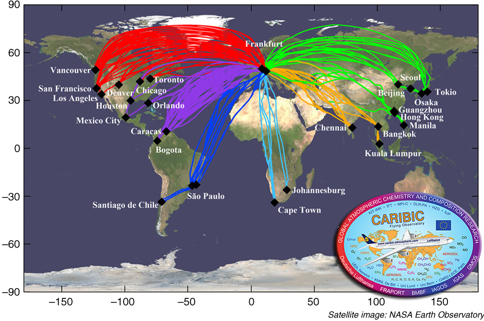
Fig. 8
IAGOS-CARIBIC map of flights (May 2005–August 2015).
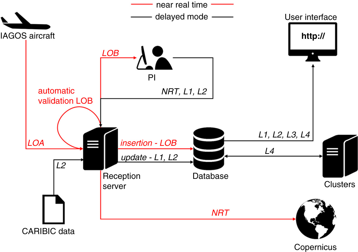
Fig. 9
Data processing path from the aircraft raw state to the user available state. Data levels refer to raw data (L0A), to automatically analysed data using pre-flight or in-flight calibrations (L0B), to data validated by the responsible PI and published as preliminary data (L1) and to final data (L2) after removal of instrument from the aircraft and post-flight calibration. Climatological data (L3) and added-value products (L4) are also available, whereas near real-time (NRT) data are made available for data assimilation and model evaluation.
Table 5. IAGOS data levels
Table 6. IAGOS database measurement products
NOx, CO2, CH4, aerosols, cloudsIAGOS-CARIBICO3, CO, H2Ogas, H2Ocloud, NO y
NO x , CO2, CH4
Particle (number) concentrations (N4–12, N12, N18, N140, M140)
Particle size distribution (140–1050 nm)
NO2
Table 7. Atmospheric state and aircraft parameters provided by the A340/A330 aircraft system
[i] Adapted from WMO (2003). aBased on the ICAO-Barometric Altitude Formula used in aviation; baltitude with respect to ground surface below aircraft; cuncertainty is here combining wind speed and direction as the vector error.
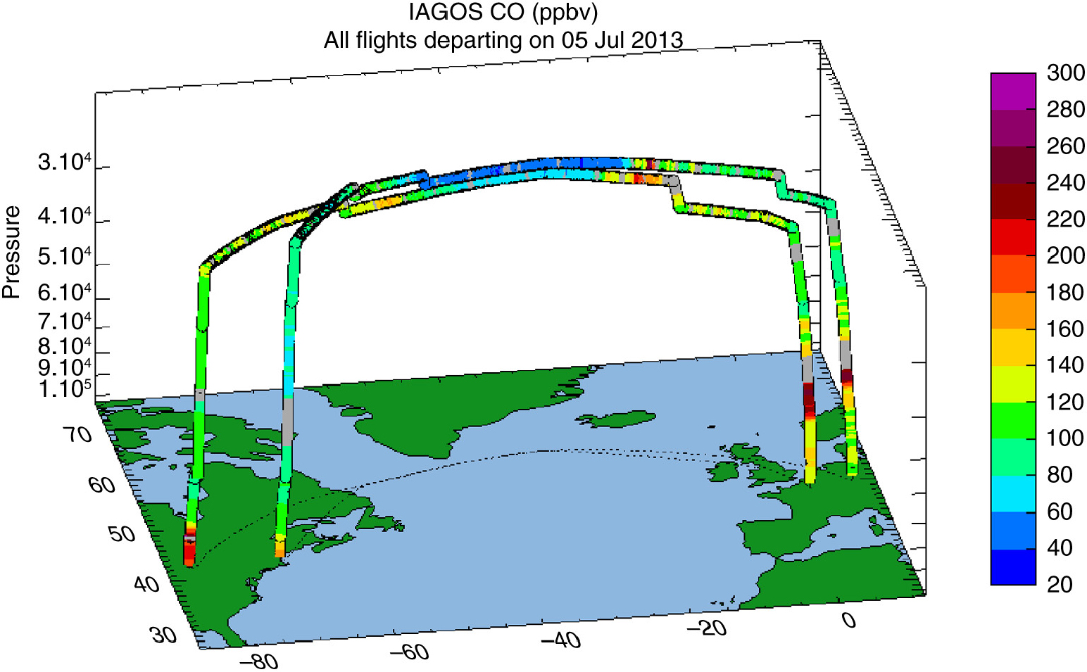
Fig. 10
Flights on 5 July 2013 showing enhanced CO at cruise altitude, in the boundary layer over the source region (North America) and in the mid-troposphere over Europe.
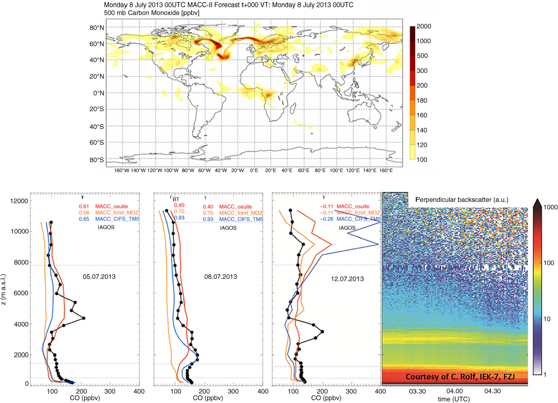
Fig. 11
Top panel: dispersion of Canadian fire plumes over Europe on 8 July 2013. Bottom panel: comparison of the vertical profiles of CO from the MACC-2 forecasts for the July 2013 episode to IAGOS measurements obtained over Frankfurt; the bottom right panel shows a LIDAR backscatter profile taken over Jülich on 12 July 2013 (adapted from Thouret and Petzold, 2015).
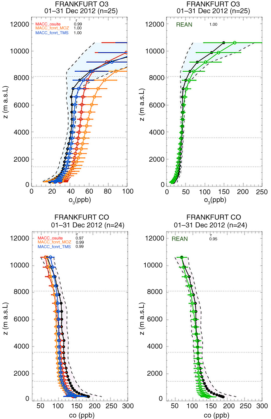
Fig. 12
Monthly mean vertical profiles of ozone (top panels) and CO (bottom panels) over Frankfurt in December 2012, as observed from MOZAIC-IAGOS (black lines) and modelled by different versions of the MACC model (coloured lines) in forecast mode (left panels) and reanalysis mode (right panel). Further examples and details may be found in www.iagos.fr/macc.
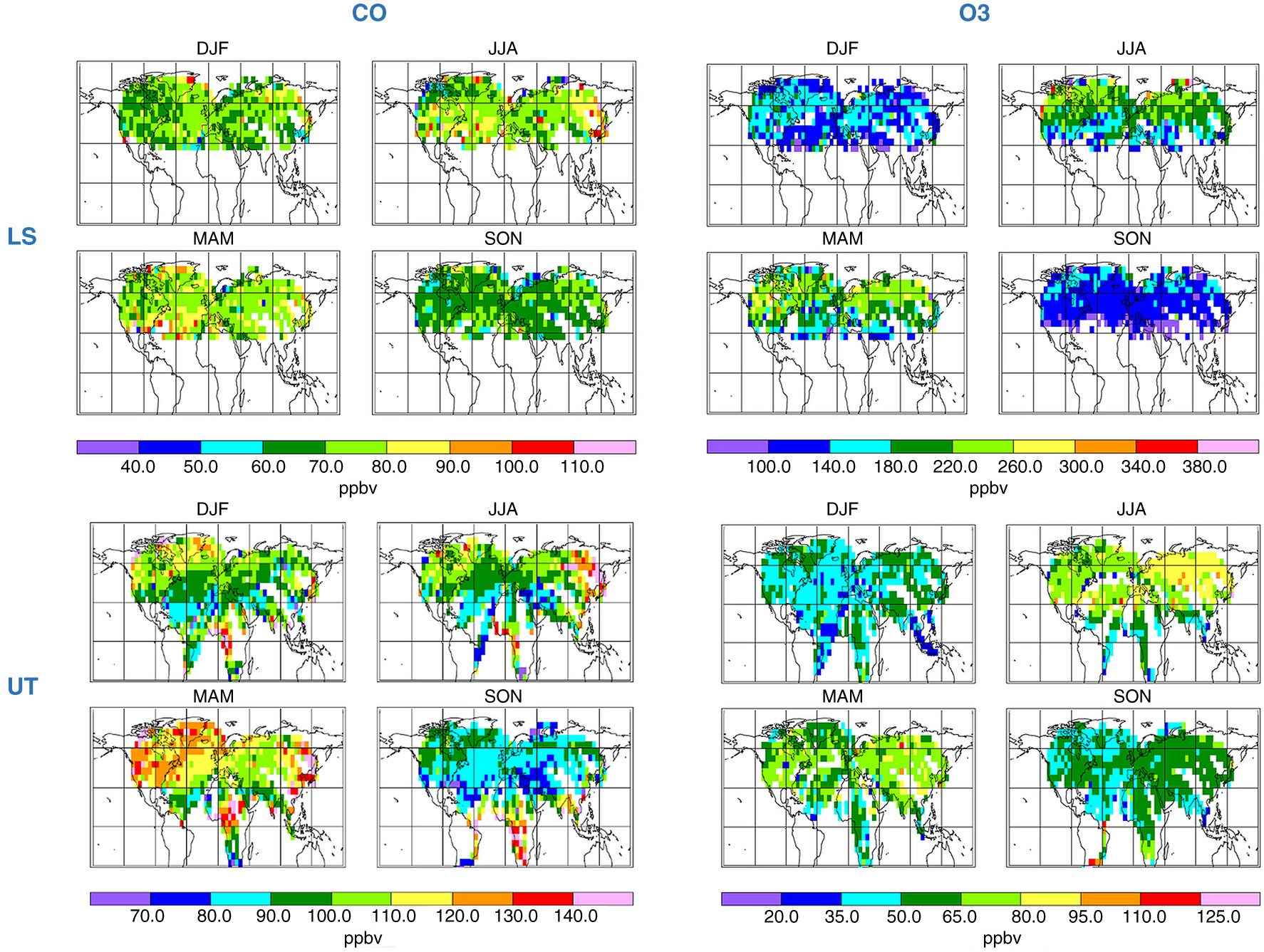
Fig. 13
CO (left panels) and ozone (right panels) seasonally averaged distributions in the UT (bottom panels) and in the LS (top panels) as recorded at cruise level by MOZAIC aircraft over the period 2001–2011. Data are averaged on 5°×5° grid cells. Lines UT display data observed between 15 and 45 hPa below the local tropopause (defined as the isoPV surface 2 pvu). Lines LS display data observed above −45 hPa above the local tropopause. Figures are adapted from Thouret et al. (2006) and extended to 2011.
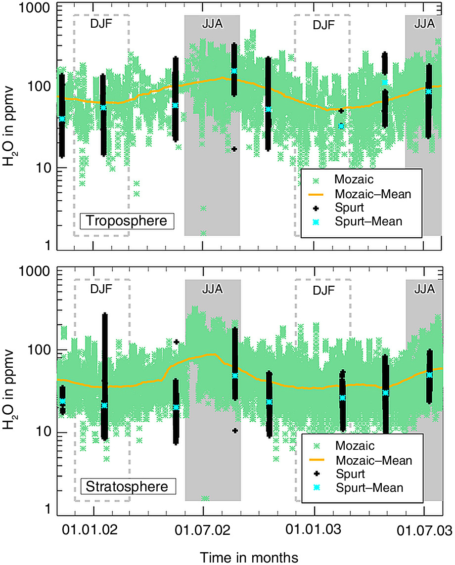
Fig. 14
Climatology of water vapour in the upper troposphere (top panel) and lowermost stratosphere (bottom panel) from SPURT and MOZAIC; courtesy of A. Kunz (2010).
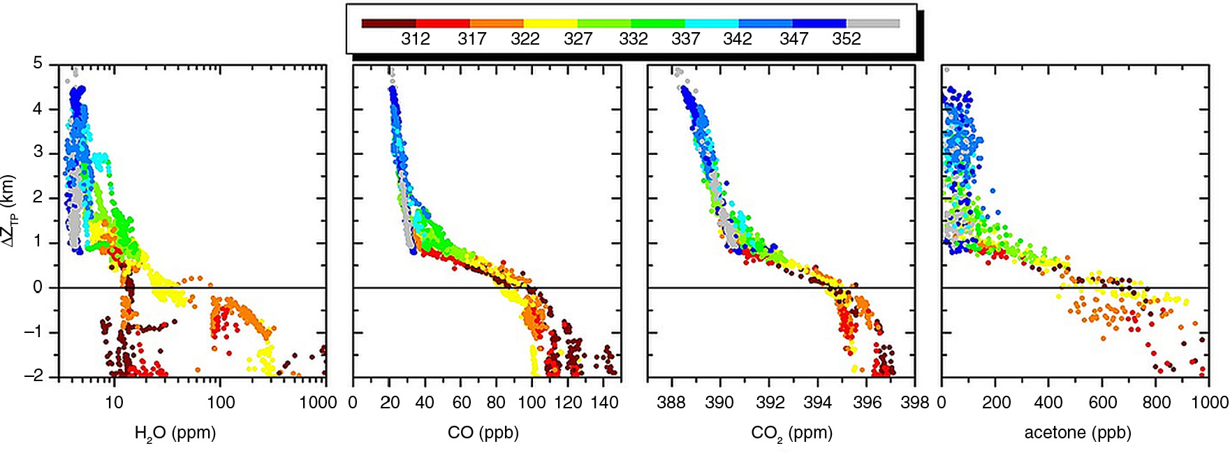
Fig. 15
Vertical profiles of H2O, CO, CO2 and acetone relative to the tropopause along a flight from Seoul (Korea) to Frankfurt (Germany) on 28 March 2012. Colour coding: potential temperature in Kelvin.