
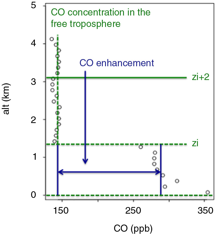
Fig. 1
Illustration of the CO enhancement in the mixed layer (height z i) above the CO in the free troposphere.
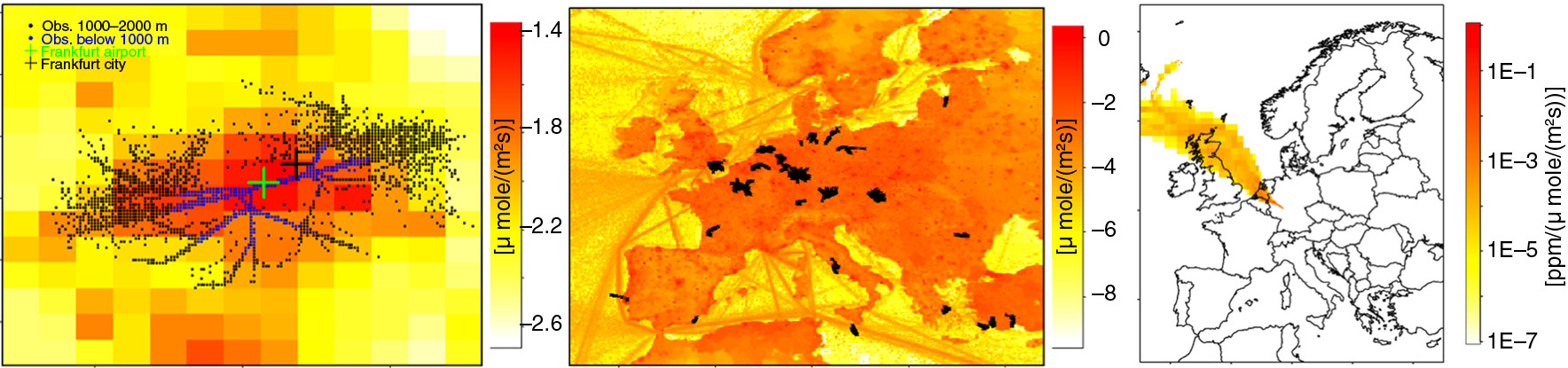
Fig. 2
MOZAIC/IAGOS flight tracks below 4 km altitude shown on a map with CO emissions based on the EDGAR version 4.3 emissions at 10 km horizontal resolution (left), MOZAIC observation locations during 2007 in the vicinity of Frankfurt, coloured by altitude (middle), and STILT/EDGAR-derived footprint (sensitivity to upstream fluxes) for a single measurement location/time near Frankfurt airport (right).
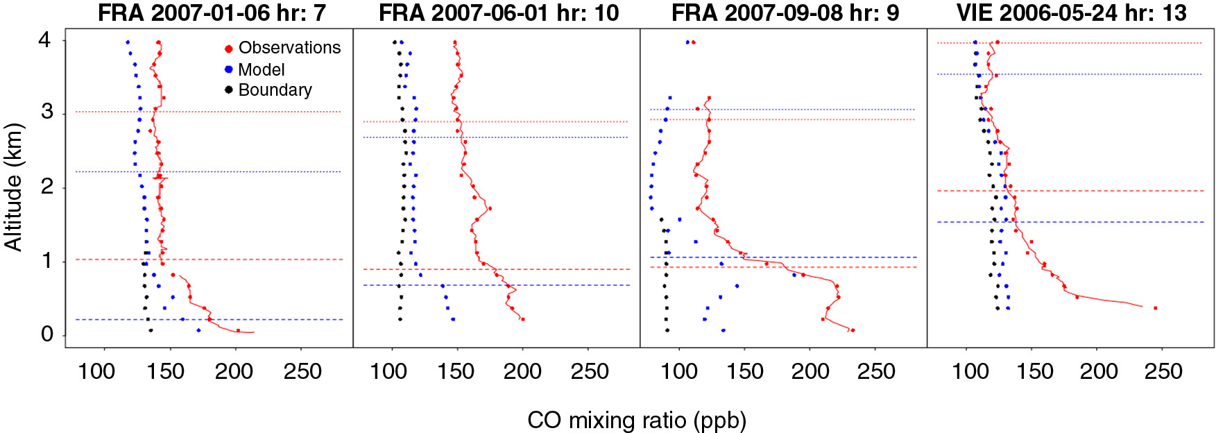
Fig. 3
Vertical profiles from MOZAIC/IAGOS observations (red), STILT/EDGAR simulations (blue) and boundary conditions from the MACC reanalysis (black) for different locations and times. Note that observations have been plotted both as continuous data (continuous red line) and averaged over 150 m intervals (red dots). The dashed lines indicate the value of z i and z i+2 km for the observed (red) and modelled (blue) profile, respectively.
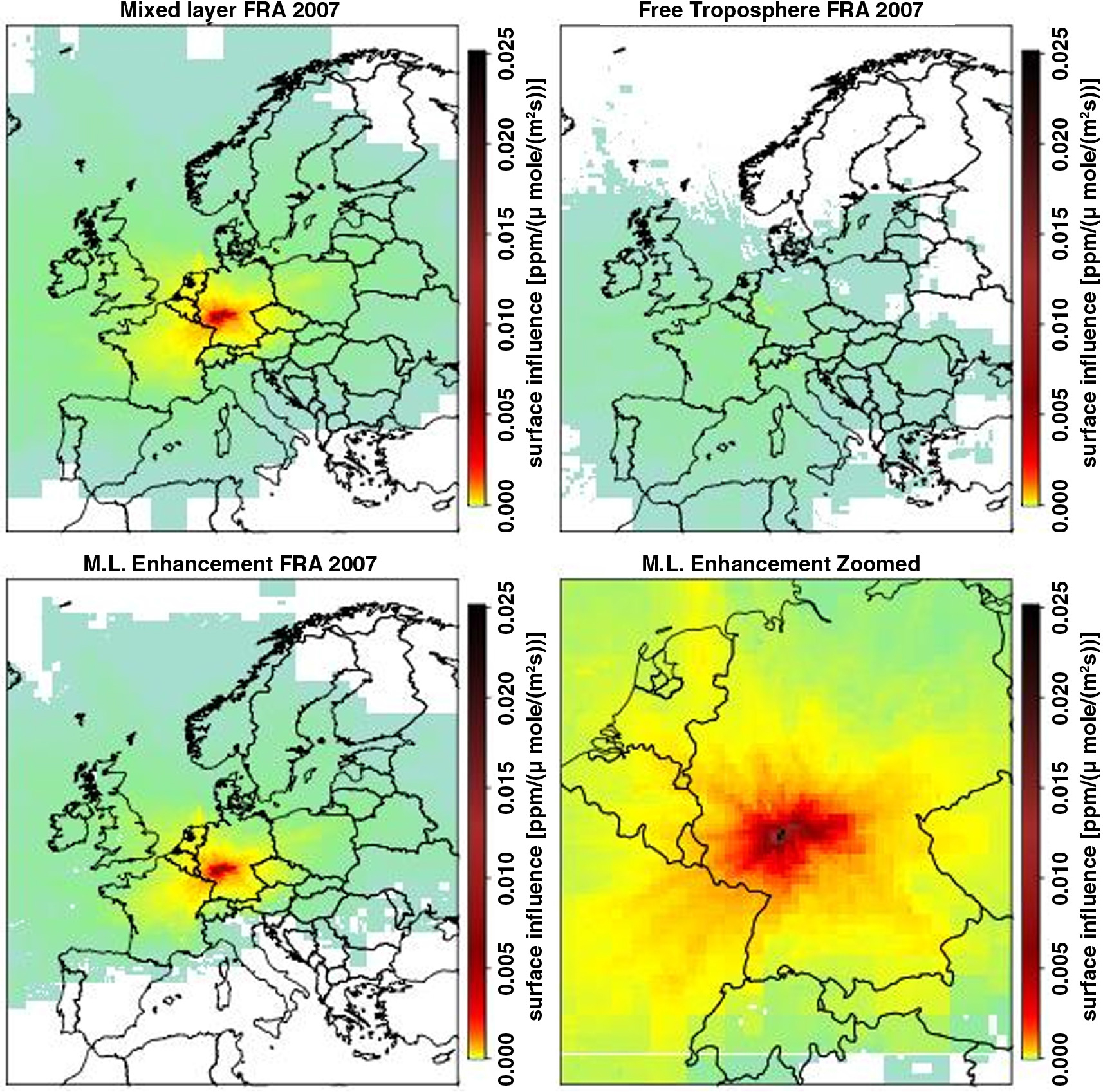
Fig. 4
Illustration for STILT-derived mean surface influence for receptor points collected near Frankfurt in 2007 for the mixed layer (top left) and free troposphere (top right). The bottom panels show the enhancements from the troposphere (the difference between the former two), with different zoom.
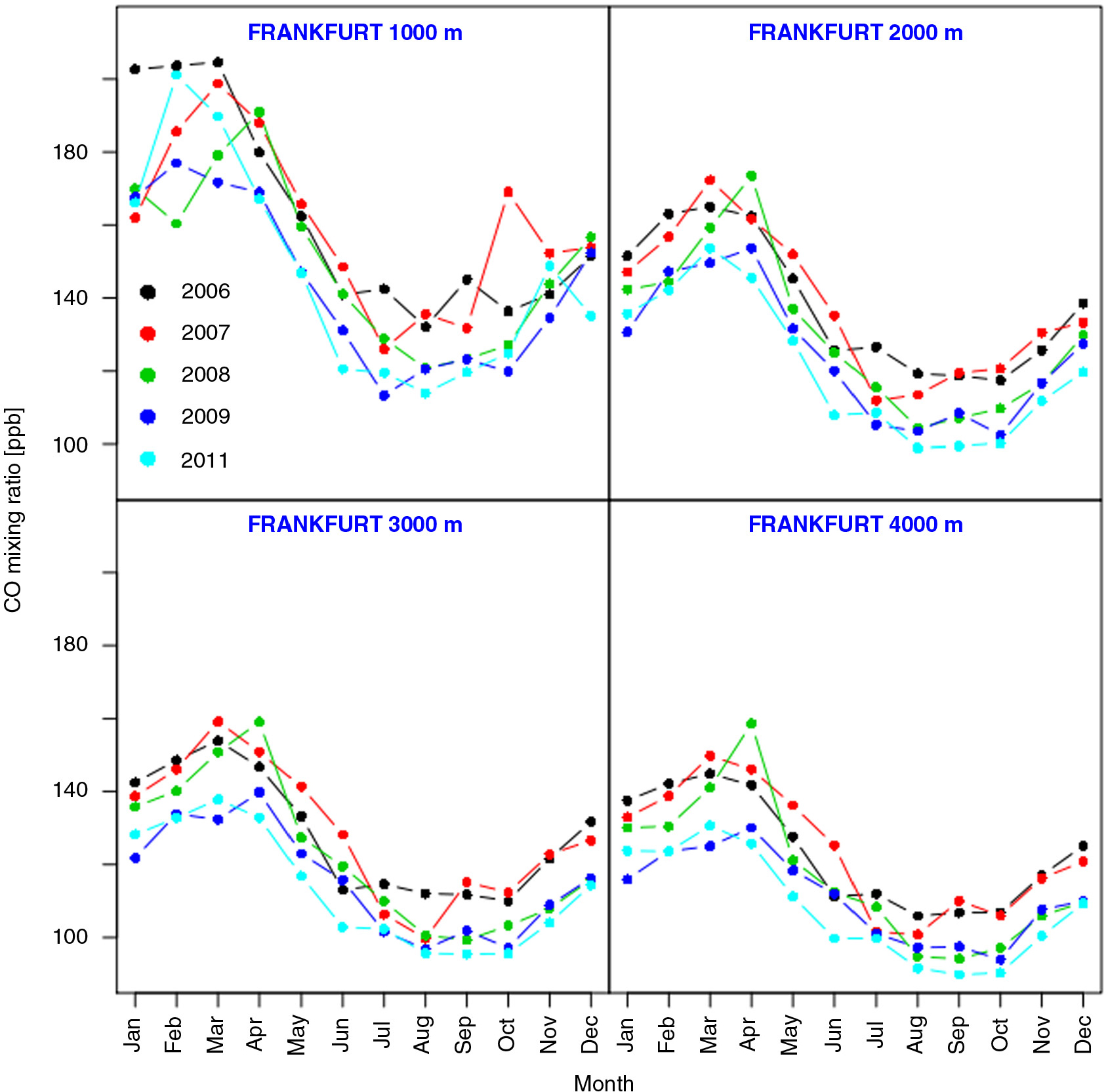
Fig. 5
Observed CO mixing ratio for the years 2006–2011 in the lower troposphere around Frankfurt. The plots show mean monthly values at four different heights. Note that values collected at 1000 m differ strongly from values collected at higher levels. In the spring (March and April) of 2007 and 2008, higher values were collected at 2000 m and above. This is likely due to an unusually high number of spring wildfires in many European countries.
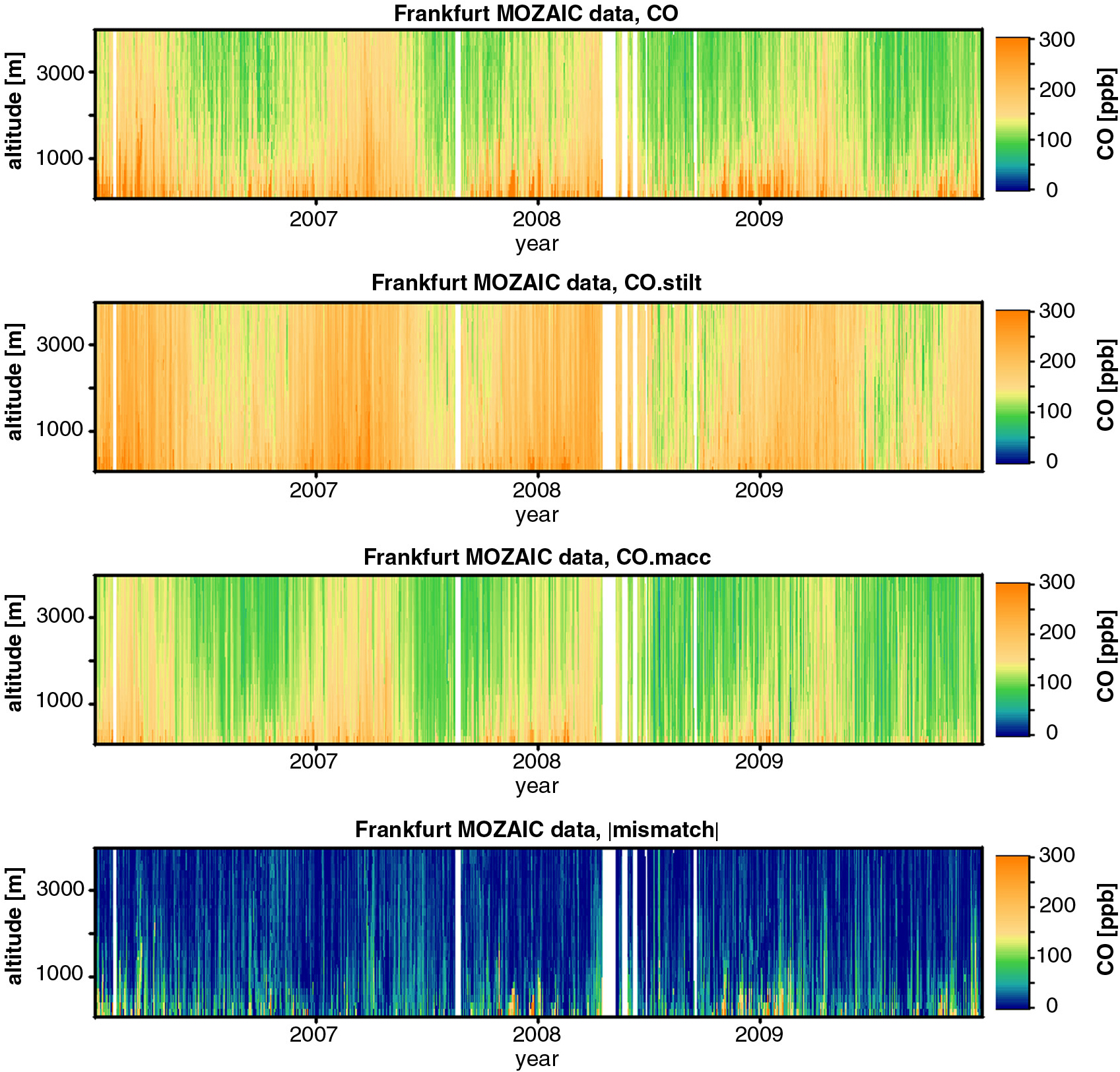
Fig. 6
Observed MOZAIC/IAGOS profiles of CO near Frankfurt (first panel, on top), together with simulated profiles of CO from STILT/EDGAR coupling and MACC reanalysis (second and third panel, respectively). The bottom panel shows the absolute value of the residuals between MOZAIC/IAGOS and MACC profiles.
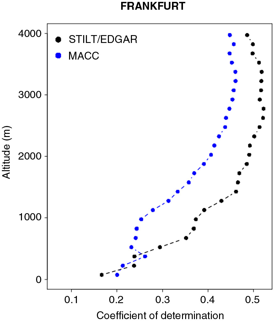
Fig. 7
Coefficient of determination (R 2) between modelled and observed CO mixing ratio for both STILT/EDGAR and MACC using profiles collected around Frankfurt's airport during 2006–2011.
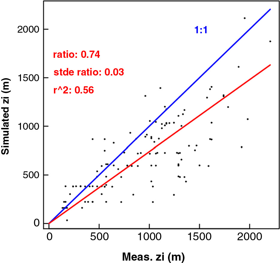
Fig. 8
Comparison of simulated vs. observation-derived mixing heights for MOZAIC profiles near Frankfurt in 2007. The red line is drawn from the origin and through the centre of mass of the scatter plot, so its slope represents the ratio of the mean simulated and observed value.
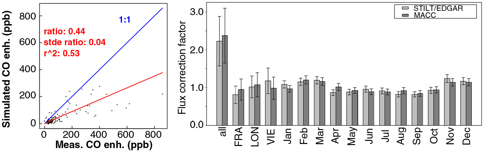
Fig. 9
In the left panel the comparison of simulated vs. observed mixed layer CO enhancements for Frankfurt profiles in 2007 during daytime (10:30–17:30 UTC) is shown. The red line is drawn from the origin and through the centre of mass of the scatter plot, so its slope represents the ratio of the mean simulated and observed value. The right panel shows the correction factors to compensate for a bias in STILT/EDGAR and MACC emission flux (right). Both correction factors and error bars (standard deviations) were derived using a weighted least-squares estimate of the parameters of a non-linear model.
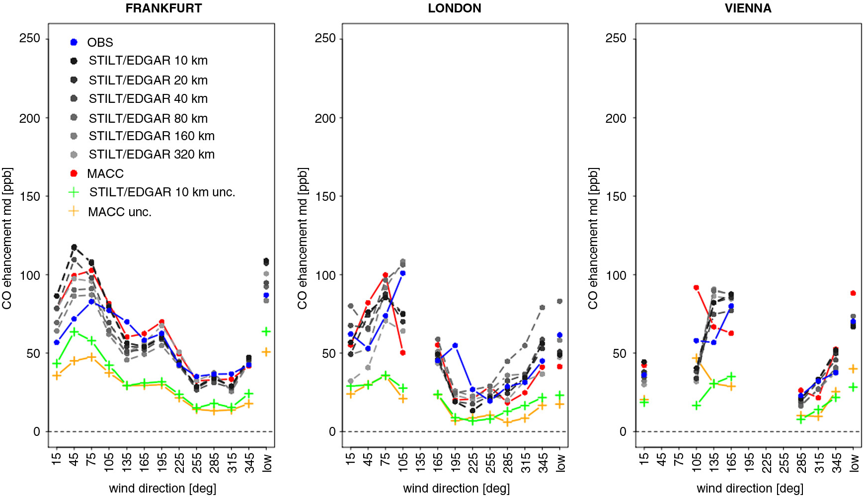
Fig. 10
Median enhancements of CO for the years 2006–2011 in the mixed layer for Frankfurt (left), London (middle) and Vienna (right), as a function of wind direction. The rightmost x-values indicated ‘low’ represent low wind speeds (<3 m/s). Observations are show in blue, STILT/EDGAR simulations in different grey tones (light for coarse, dark for high resolution), and MACC reanalysis results are shown in red. STILT/EDGAR and MACC uncorrected enhancements are shown in green and ochre, respectively.
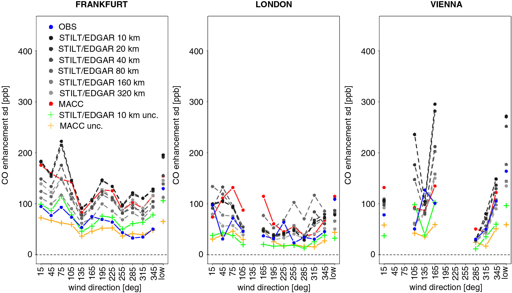
Fig. 11
As Fig. 10, but for the standard deviation of the enhancements of CO for the different wind sectors.
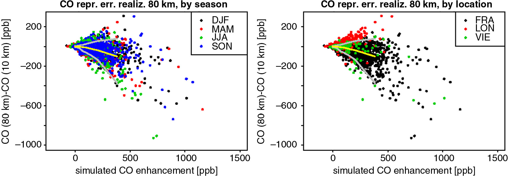
Fig. 12
Realisations of representation error (i.e. differences between STILT simulations at different resolutions, here 10 and 160 km) for CO plotted against simulated enhancement, and colour-coded by season (left) and by airport location (right). Grey lines indicate the 5th and 95th percentile of the distribution within 10 bins of simulated enhancement; the yellow line indicates the mean.
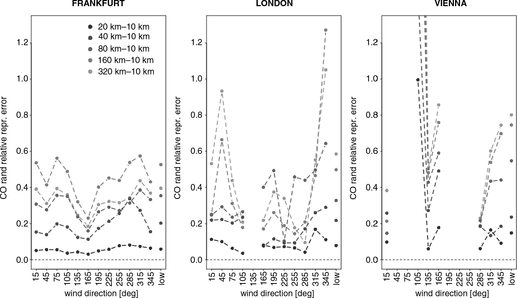
Fig. 13
Random component of the relative representation error for CO for the years 2006–2011 in the mixed layer for Frankfurt (left), London (middle) and Vienna (right), as a function of wind direction. The rightmost x-values indicated ‘low’ represent low wind speeds (<3 m/s). STILT/EDGAR simulations are shown in different grey tones (light for coarse, dark for high resolution). Maximum relative error for Vienna at 105 degrees is up to 4.8.
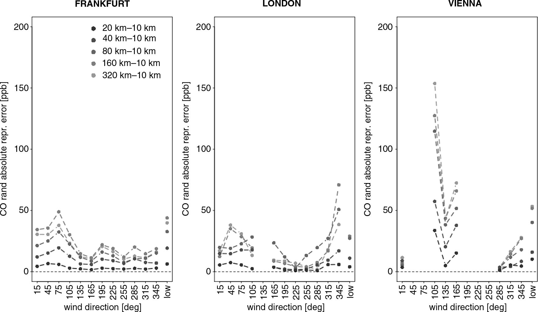
Fig. 14
As Fig. 13, but for absolute representation error.
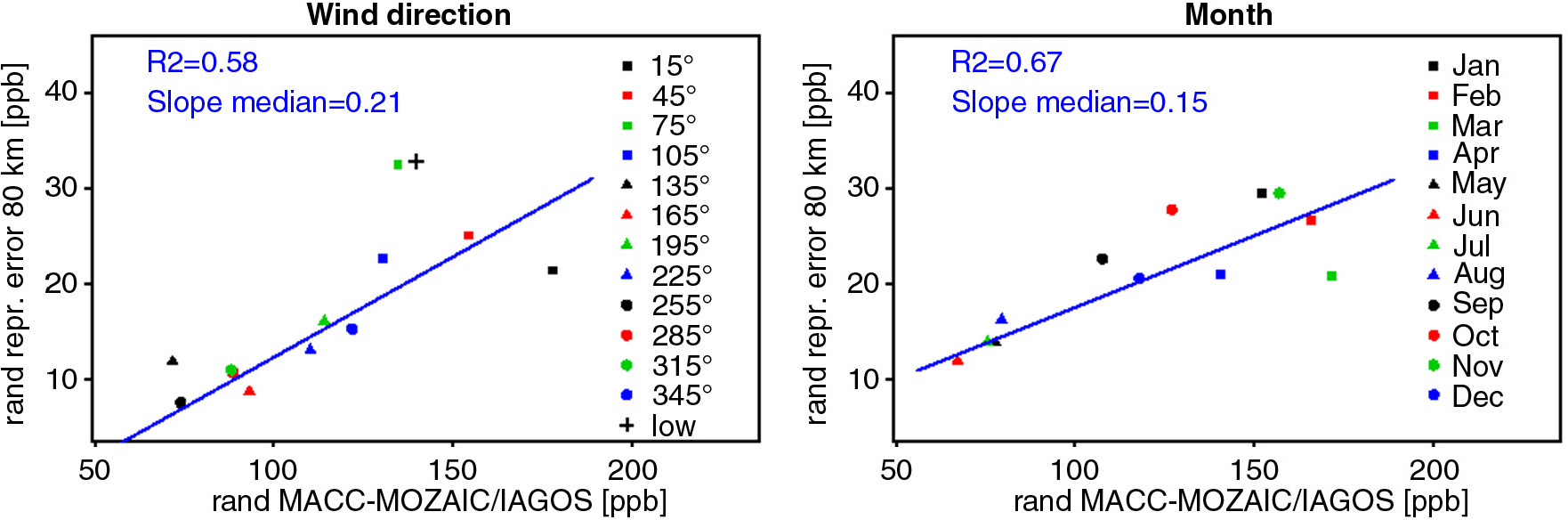
Fig. 15
Random component for representation error of Frankfurt for different wind directions (left) and months (right), plotted against the corresponding model–data mismatch error.
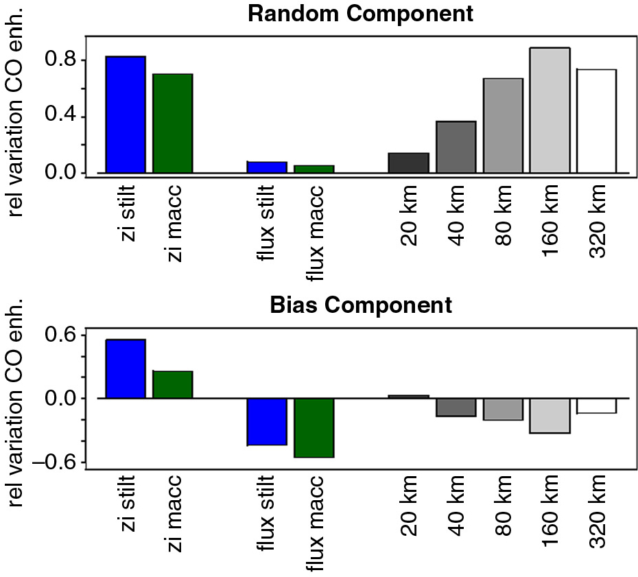
Fig. 16
Assessment of contribution of different error categories for the city of Frankfurt. The assessment is treated separately for random (upper tab) and bias (lower tab) component. For each component the uncertainty of the correction for mismatch in the mixing height (z i) and bias in the emission inventories (flux) is shown for both STILT (left) and MACC (centre) models; the contribution from the spatial resolution of EDGAR fluxes to STILT/EDGAR uncertainty is shown for each of the considered resolutions (right).
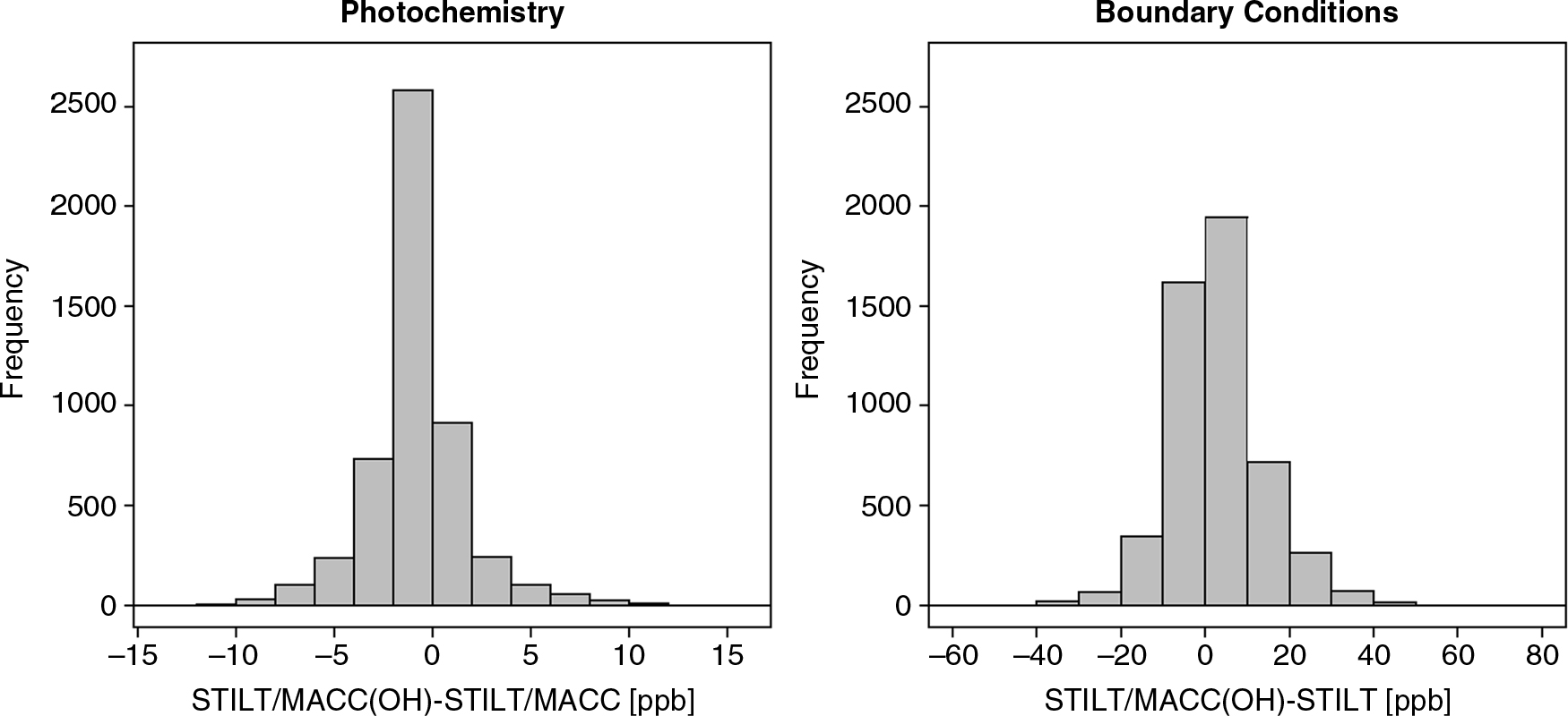
Fig. 17
Absolute change in CO enhancements due to photochemistry (left) and boundary condition (right) on the whole dataset. Standard deviation of residuals is quantified as 2.6 ppb for photochemistry and 11.1 ppb for the boundary condition. Note the different scale on the x-axis of the two plots.