
Table 1. Summary of tropospheric ozone measurements available in databases
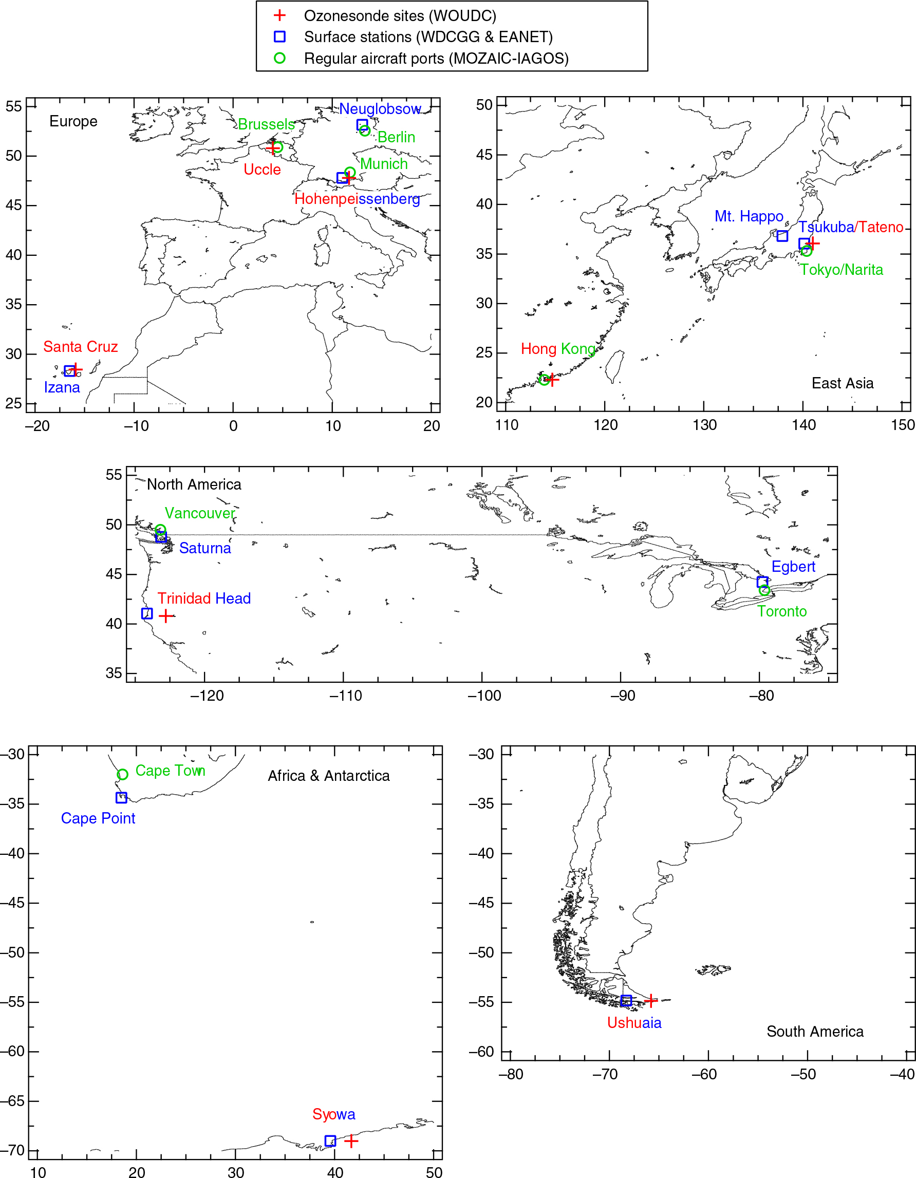
Fig. 1
Global distribution of the sites of sonde, surface and regular aircraft observations examined in this work.
Table 2. Characteristics of the sites measuring tropospheric ozone, relevant for the sonde and surface comparisons
WOUDC STNSurface
WDCGG ID Distance (km) PeriodNumber of matched hourly dataGermanyHohenpeissenberg (976 m)99Hohenpeissenberg (985 m)HPB~01995–2007BM: 1598JapanTateno/Tsukuba (31 m)14Tsukuba (25 m)TKB~01988–20121115 (CI: 989, ECC: 126)JapanSyowa (22 m)101Syowa (16 m)SYO~01999–2012720 (CI: 631, ECC: 89)SpainSanta Cruz (36 m)401Izana (2367 m)IZO~272008–2012ECC: 291ArgentinaUshuaia (17 m)339Ushuaia (18 m)USH~01996–2003ECC: 126USATrinidad Head (107 m)445Trinidad Head (120 m)THD~282004–2006ECC: 85
Table 3. Effects of correction factor (CF) on the agreement between ozonesonde measurements and surface observations of tropospheric ozone
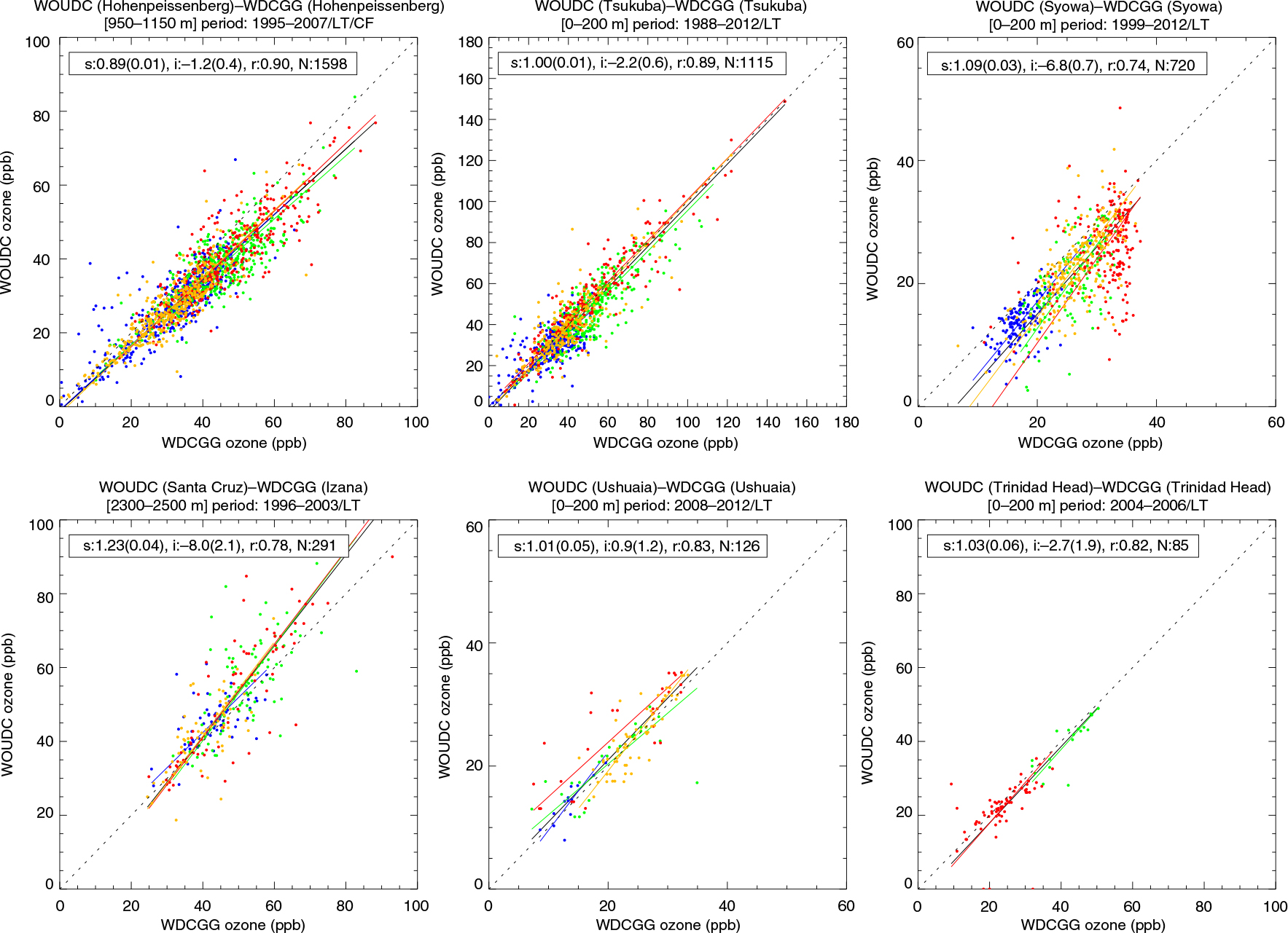
Fig. 2
Scatter plots of tropospheric ozone mixing ratios measured by sondes versus those measured at surface sites. The data and regression lines for winter (DJF), spring (MAM), summer (JJA) and fall (SON) are illustrated with blue, green, red, and orange symbols, respectively. The regression line for all the data is illustrated in black, and its slope (s), intercept (i), correlation coefficient (r) and data number (N) are denoted with the associated 95% confidence level. The correction factor (CF) is applied to the ozonesonde data at Hohenpeissenberg, but not at the other five sites.
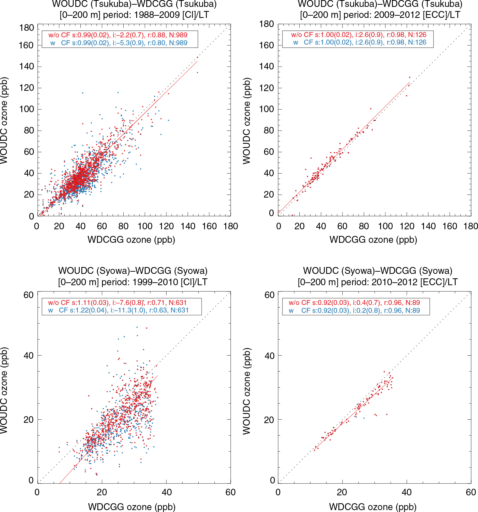
Fig. 3
Same as Fig. 2 but for different sensor types for sondes [left, Carbon Iodine (CI); right, Electro-chemical Concentration Cell (ECC)] in Tsukuba (top panel) and Syowa (bottom panel). The plots show the data both with CF (blue) and without CF (red).
Table 4. Characteristics of the sites where tropospheric ozone is measured, relevant for the aircraft and surface comparisons
MOZAIC-IAGOS IATASurface
WDCGG ID Distance (km) PeriodNumber of matched hourly dataGermanyMunich (453 m)MUCHohenpeissenberg (985 m)HPB841996–20062059JapanTokyo/Narita (43 m)NRTTsukuba (25 m)TKB401995–20121113CanadaToronto (173 m)YYZEgbert (253 m)EGB621994–2003271CanadaVancouver (4 m)YVRSaturna (178 m)SAT461998–2003135South AfricaCape Town (46 m)CPTCape Point (230 m)CPT441998–200957GermanyBerlin (37 m)TXLNeuglobsow (65 m)NGL701994–200437
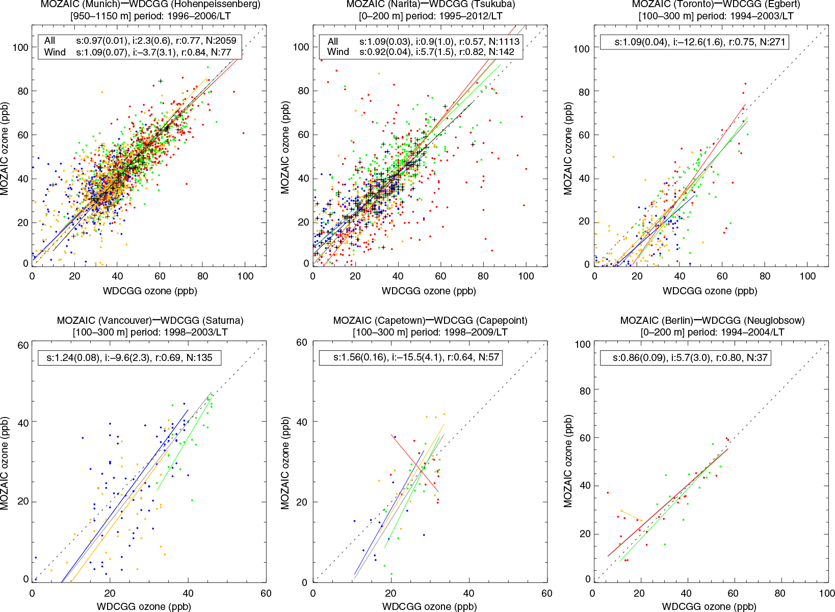
Fig. 4
Scatter plots of tropospheric ozone mixing ratios measured by regular aircraft versus those measured at surface sites. Plus symbols indicate the data pairs after wind selection.
Table 5. Characteristics of the sites where tropospheric ozone is measured, relevant for the aircraft and sonde comparisons
MOZAIC-IAGOS IATASonde
WOUDC STN Distance (km) PeriodNumber of matched hourly dataaBelgiumBrussels (56 m)BRUUccle (100 m)53201997–2009ECC: 566GermanyMunich (453 m)MUCHohenpeissenberg (976 m)99841998–2006BM: 327JapanTokyo/Narita (43 m)NRTTateno/Tsukuba (31 m)14401996–201298 (CI: 97, ECC: 1)Hong KongHong Kong (9 m)HKGHong Kong (66 m)344282000–201020
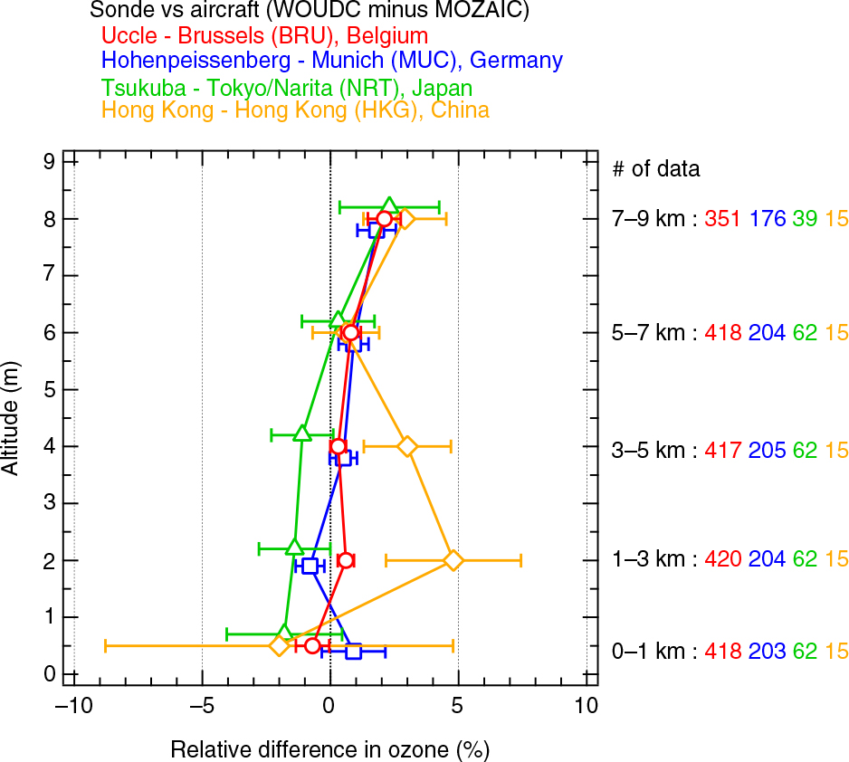
Fig. 5
Medians of the relative differences in tropospheric ozone mixing ratios for five altitude levels measured by sondes and regular aircraft. Error bars denote the 95% confidence level.
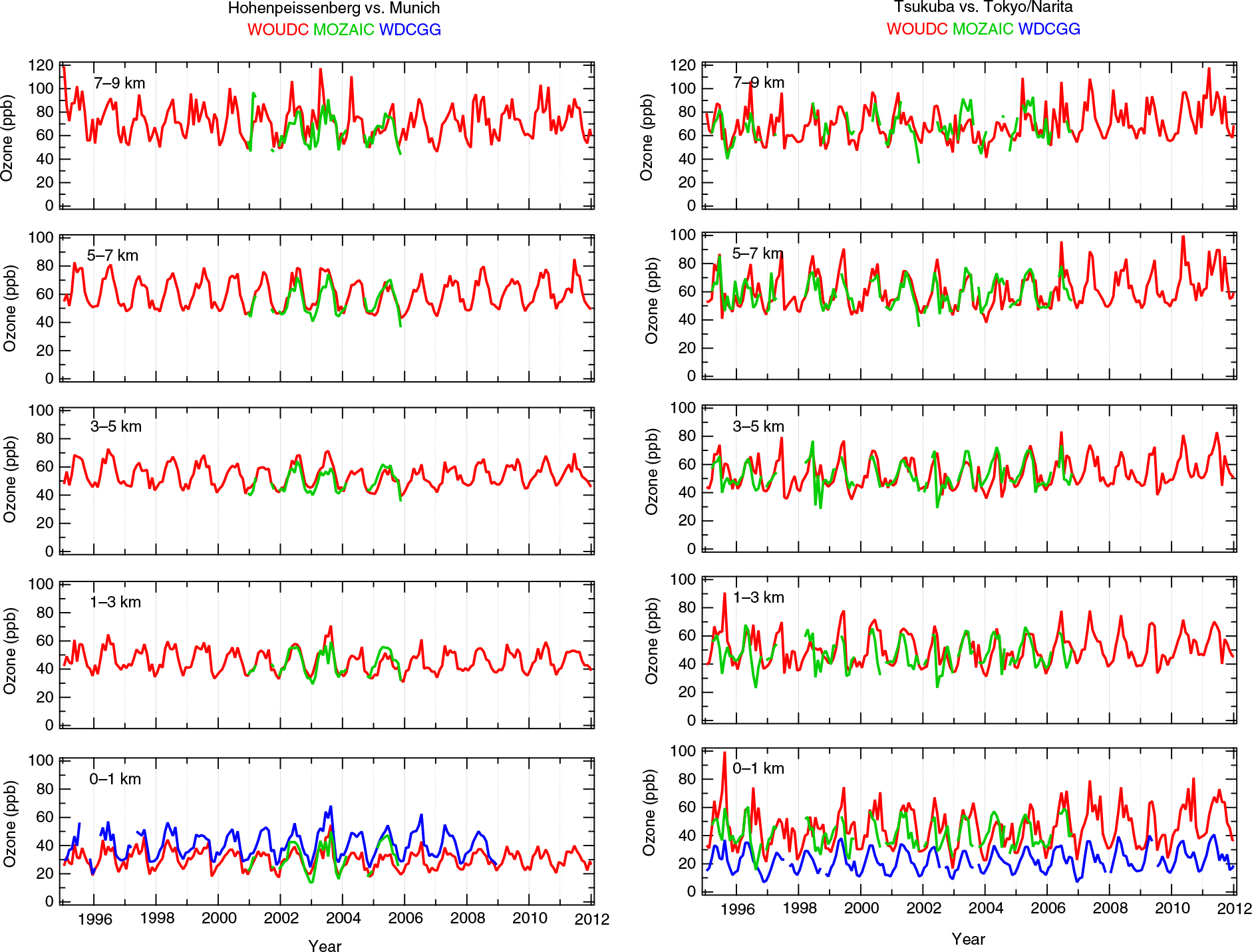
Fig. 6
Time series of tropospheric ozone mixing ratios measured by sondes, regular aircraft and at surface stations for five altitude levels in the troposphere at Hohenpeissenberg (left) and Tsukuba (right).
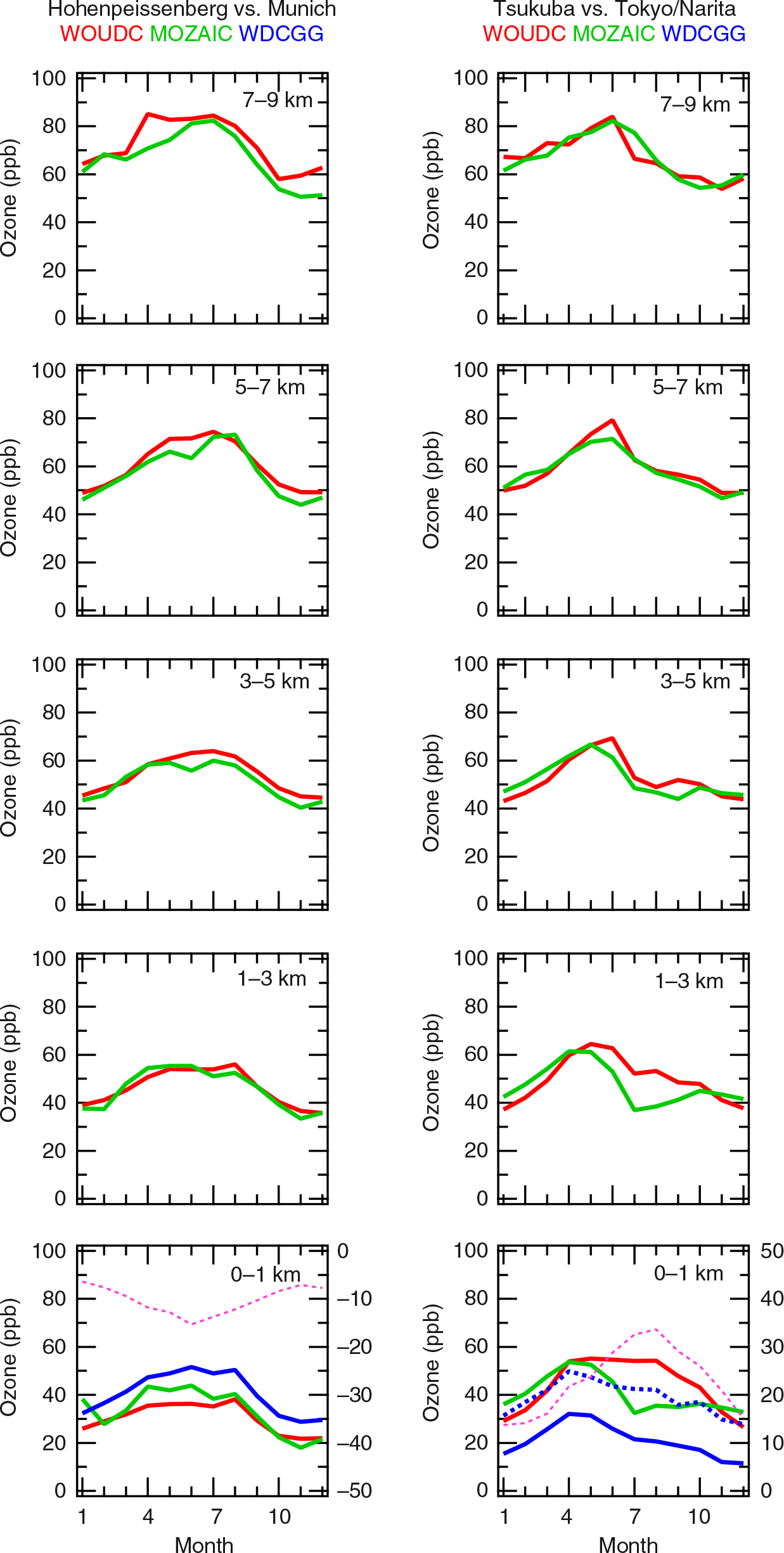
Fig. 7
Seasonal cycles of tropospheric ozone mixing ratios measured by sondes, regular aircraft and at surface stations at different altitudes at Hohenpeissenberg (left) and Tsukuba (right). The sonde-minus-surface differences in O3 are expressed by pink dotted lines for the right axis. The dashed blue line in Tsukuba shows the seasonal cycle of the surface observations based only on the 14:00–15:00 LT data.
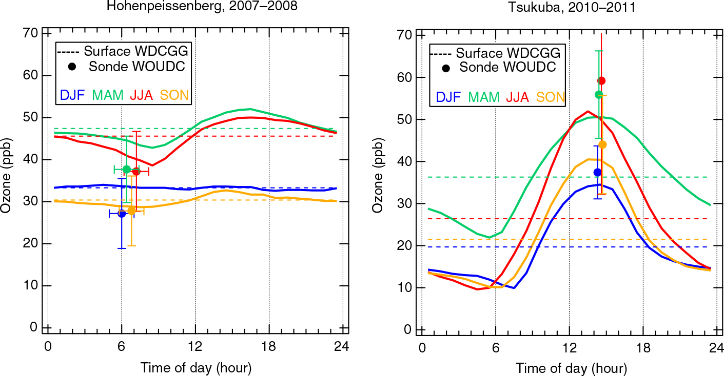
Fig. 8
Mean diurnal cycles of tropospheric ozone mixing ratios at the surface level in Hohenpeissenberg and Tsukuba, as measured using surface stations and sondes. Vertical error bars denote one standard deviation and horizontal error bars for Hohenpeissenberg denote the range of time for the sonde launching. Dashed lines are daily means calculated from the surface data.
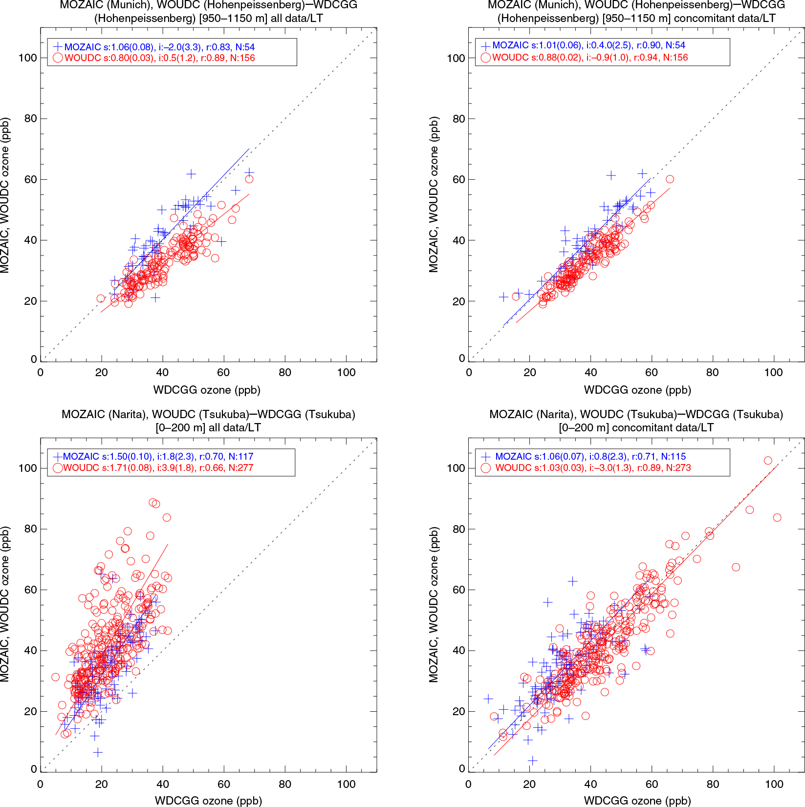
Fig. 9
Scatter plots of monthly mean ozone measured by sondes, regular aircraft and surface stations, made of all (left) and concomitant (right) hourly data at Hohenpeissenberg (top panel) and Tsukuba (bottom panel).
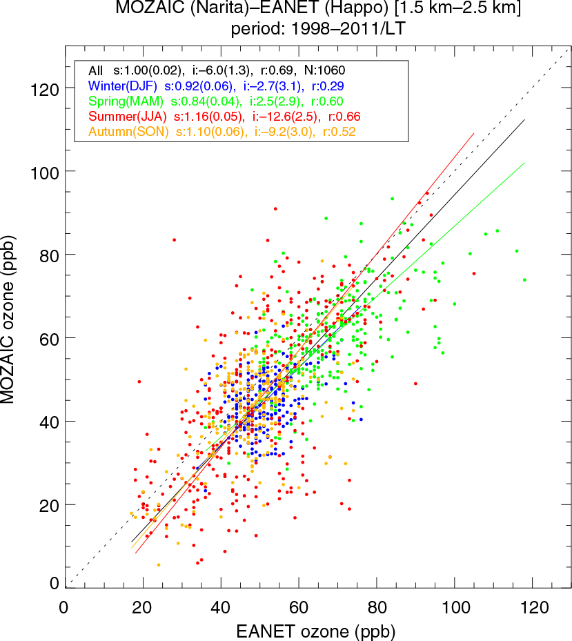
Fig. 10
Scatter plots of concomitant data sets of hourly mean ozone measurements at Mt. Happo and over Tokyo/Narita for the altitude of 1.5–2.5 km. The data and regression lines for winter (DJF), spring (MAM), summer (JJA) and fall (SON) are illustrated by blue, green, red and orange symbols, respectively. The regression line for all the data is illustrated in black, and its slope (s), intercept (i), correlation coefficient (r) and data number (N) are denoted with the associated 95% confidence level.
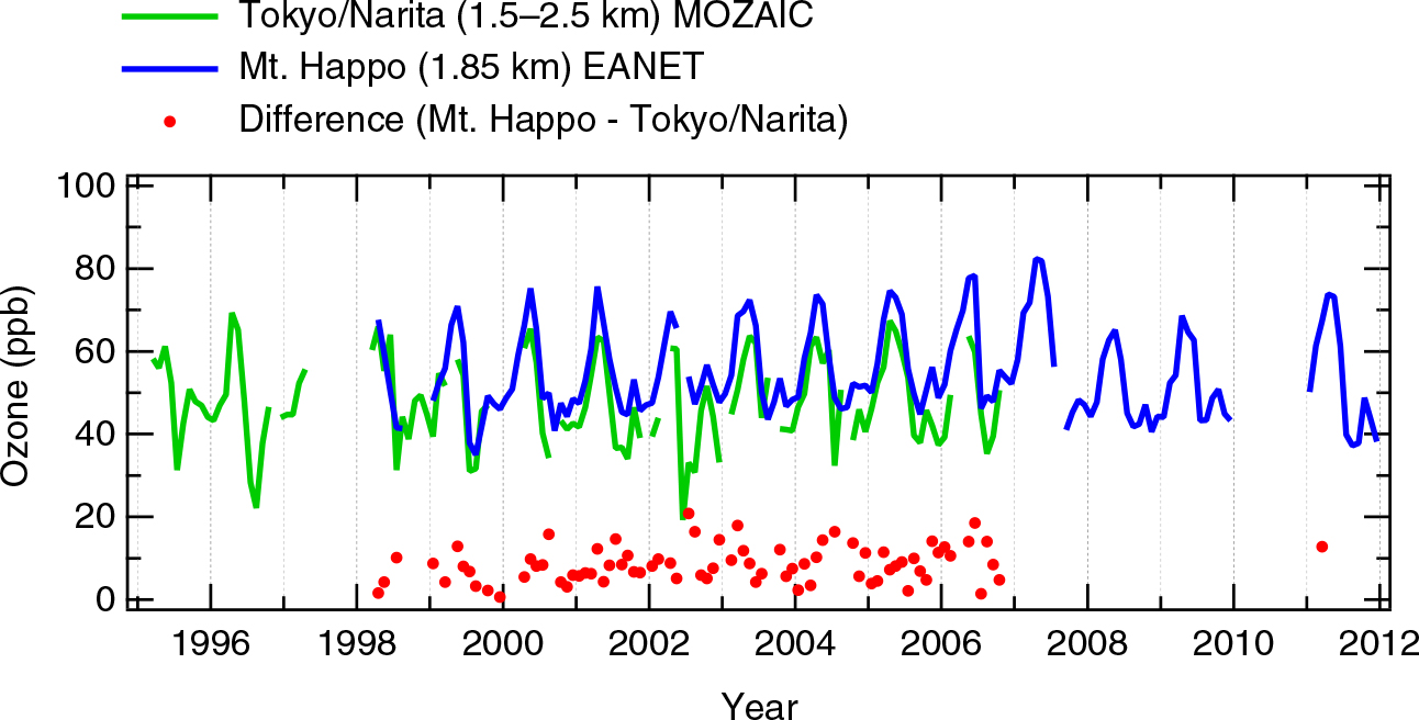
Fig. 11
Time series of monthly mean ozone observed at Mt. Happo and over Tokyo/Narita for the altitude of 1.5–2.5 km. The differences between two observations sites (Mt. Happo minus Tokyo/Narita) are also plotted.
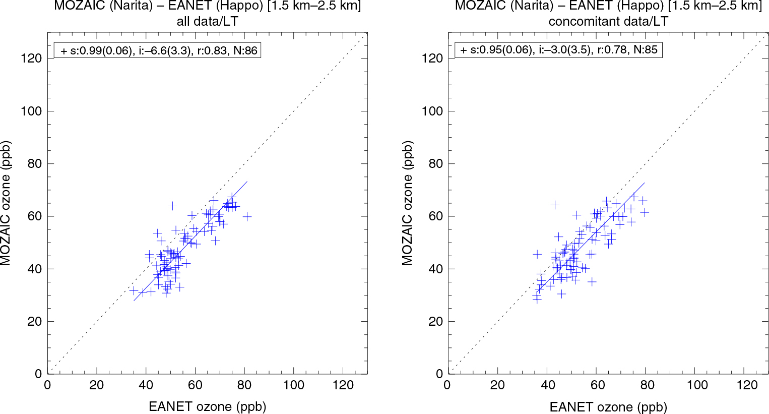
Fig. 12
Scatter plots of monthly mean ozone made of all (left) and concomitant (right) hourly data, at Mt. Happo and over Tokyo/Narita for the altitude of 1.5–2.5 km.