
Table 1. Total amount of SO2 (Tg) emitted for each of the 4-d long eruption, and its vertical distribution
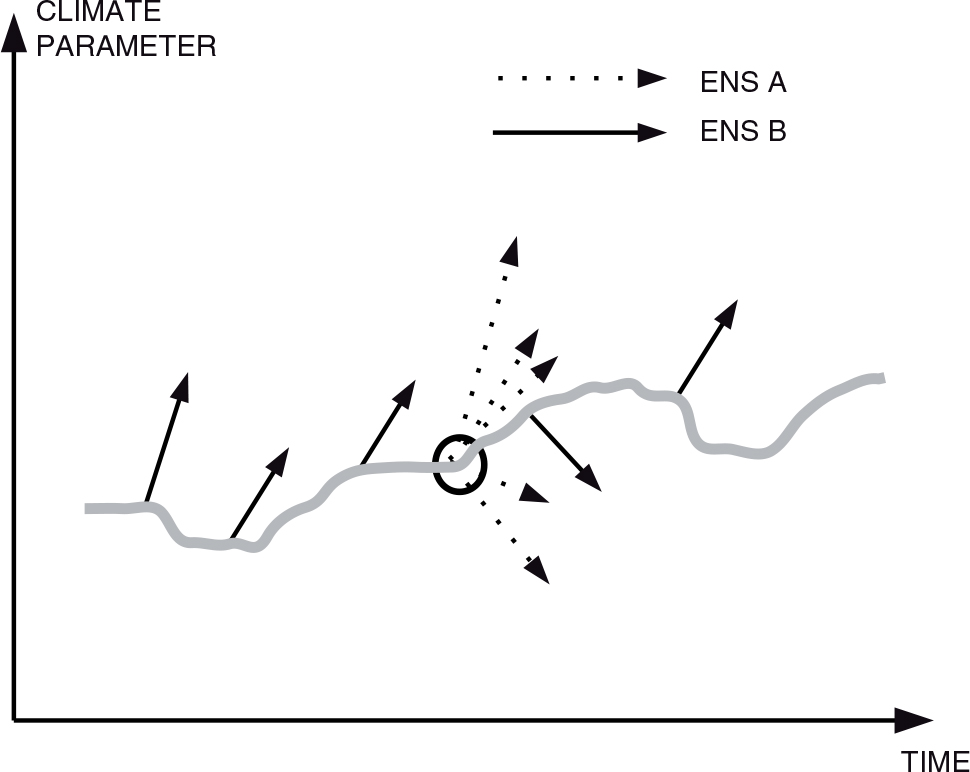
Fig. 1
Schematic representation of the two different ensembles used in this study. The dotted arrows show ENS–A that is generated starting each member from the same background state; the solid arrows show ENS–B that is generated starting each member from a different background state.
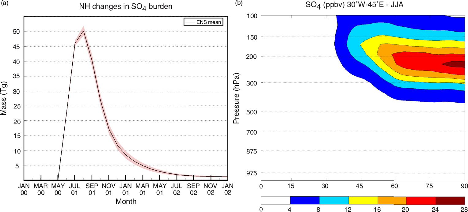
Fig. 2
Ensemble mean change (ENSvolc–A minus ENSno-volc–B) in SO4 (Tg) mass loading (left) and 30°W to 45°E mean SO4 concentrations (ppbv) for the summer of the eruption (JJA year 01) over the Northern Hemisphere (NH) from the surface to 100 mbar (right). The 30°W to 45°E interval has been chosen for direct comparison to Fig. 8 in Oman et al. (2006b). The shading in the left panel represents the standard deviation of the ensemble difference.
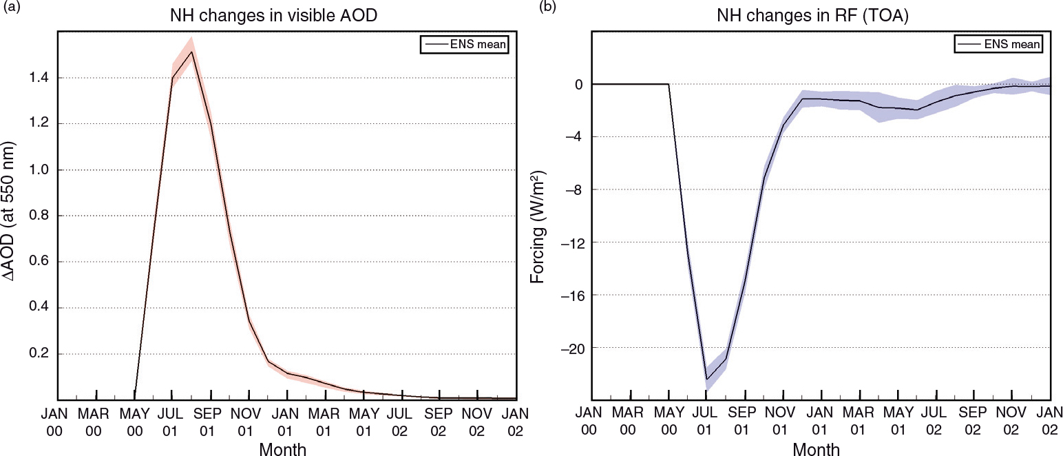
Fig. 3
Ensemble mean change (ENSvolc–A minus ENSno-volc–B) in NH visible (550 nm) aerosol optical depth – AOD (left) and net radiative forcing (shortwave + longwave) at the top of the atmosphere – TOA (right) due to a Laki-type volcanic eruption. The shadings represent the standard deviation of the ensemble difference.
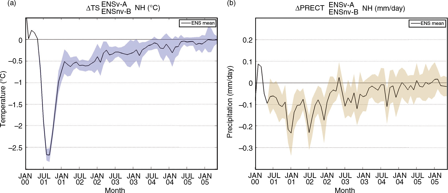
Fig. 4
Ensemble mean change (ENSvolc–A minus ENSno-volc–B) in NH surface temperature – TS (left) and precipitation – PRECT (right). The shadings represent the standard deviation of the ensemble difference.
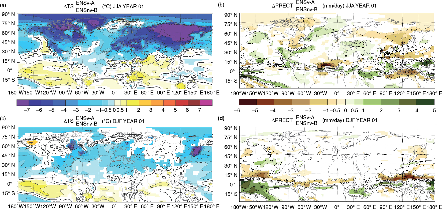
Fig. 5
Ensemble mean change (ENSvolc–A minus ENSno-volc–B) in surface temperature – TS (left) and in precipitation – PRECT (right) for the summer (JJA, upper panels) and winter (DJF, lower panels) of the year of the eruption. The colour shading displays significant anomalies at 95% confidence level. The contour intervals (dashed=negative anomalies; solid=positive anomalies) follow the colour bar scale. The bold line indicates the 0°C anomaly.
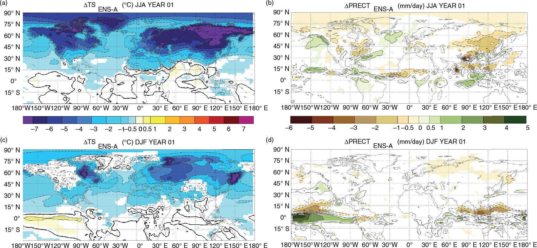
Fig. 6
Ensemble mean change (ENSvolc–A minus ENSno-volc–A) in surface temperature – TS (left) and in precipitation – PRECT (right) for the summer (JJA, upper panels) and winter (DJF, lower panels) following the eruption. The colour shading displays significant anomalies at 95% confidence level. The contour intervals (dashed=negative anomalies; solid=positive anomalies) follow the colour bar scale. The bold line indicates the 0°C anomaly.
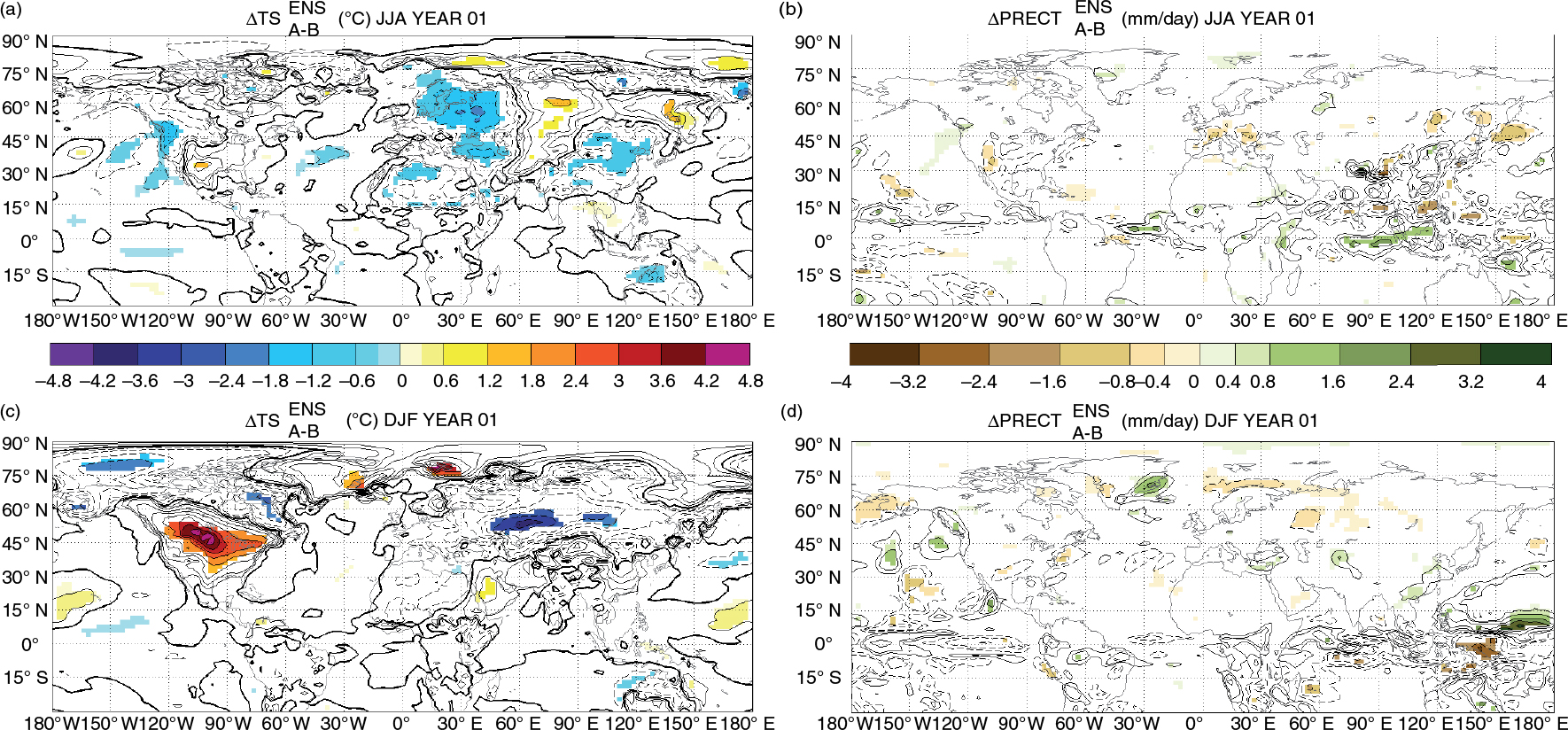
Fig. 7
Differences in surface temperature – TS (left) and precipitation – PRECT (right) anomalies for the summer (JJA, upper panels) and winter (DJF, lower panels) following the eruption between the two different approaches [e.g. ΔTS(ENS–A) – ΔTS(ENS–B)]. The contour intervals (dashed=negative anomalies; solid=positive anomalies) follow the colour bar scale. The bold line indicates the 0°C anomaly. The colour shading displays significant differences at 95% confidence level.
Table 2. Land-surface temperature SEMs (°C) for ENSno-volc and its relative changes (in %) for ENSvolc for the summer (JJA) and the winter (DJF) of the year of the eruption in both ensemble set-ups
ENS–ASEMTS (°C)
ENS–BJJADJFJJADJFNorth AmericaENSno-volc0.310.980.382.09ENSvolc+50%+18%+22%−27%EuropeENSno-volc0.401.030.441.04ENSvolc+11%+45%+23%+19%AsiaENSno-volc0.461.490.361.13ENSvolc−11%+4%+35%+30%
Table 3. Changes in land-surface temperature (°C) relative to ENSno-volc–A for the summer (JJA) and the winter (DJF) of the year of the eruption in the ENSvolc–A and the sensitivity experiments (ENSredv and ENSfixv)
ENSvolc–AΔTS (°C)
ENSredvolc–AΔTS (°C)
ENSfixvolc−AJJADJFJJADJFJJADJFNorth America−4.61−1.43−1.41−0.16−3.81+0.16Europe−4.66−2.16−1.51−0.96−3.78−1.10Asia−5.73−2.45−2.00−1.28−4.49−1.03
Table 4. Changes (in %) in land-surface temperature SEMs (°C) relative to ENSno-volc–A for the summer (JJA) and the winter (DJF) of the year of the eruption in the sensitivity experiments (ENSredv and ENSfixv) for the ENS–A set-up
ENSredvolc–AΔSEMTS (°C)
ENSfixvolc–AJJADJFJJADJFNorth America+32%+29%+22%−15%Europe−4%+33%+10%+18%Asia+65%+18%−19%+2%
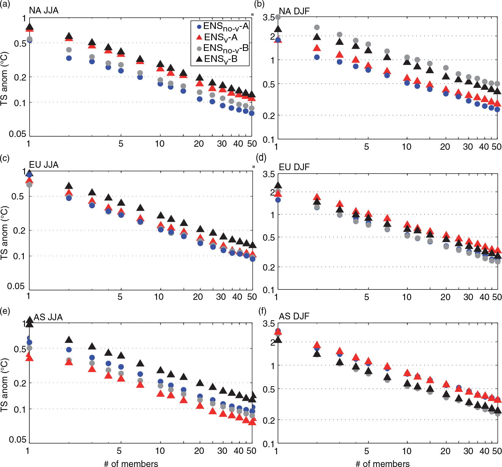
Fig. 8
Average between the absolute values of 5th and 95th percentile of distributions as a function of the number of ensemble members (n) for North America (NA), Europe (EU) and Asia (AS) for the summer (JJA) and winter (DJF) of the eruption, calculated for each ensemble. The 5th and 95th anomalies are fairly symmetric around the mean for a number of members greater than 5: The difference in absolute value between the 5th and 95th percentiles is below 0.1°C. The curves show the temperature anomalies that can be detected at the 95% confidence level as a function of n. The anomalies are computed relative to the all-member mean of each ensemble.