
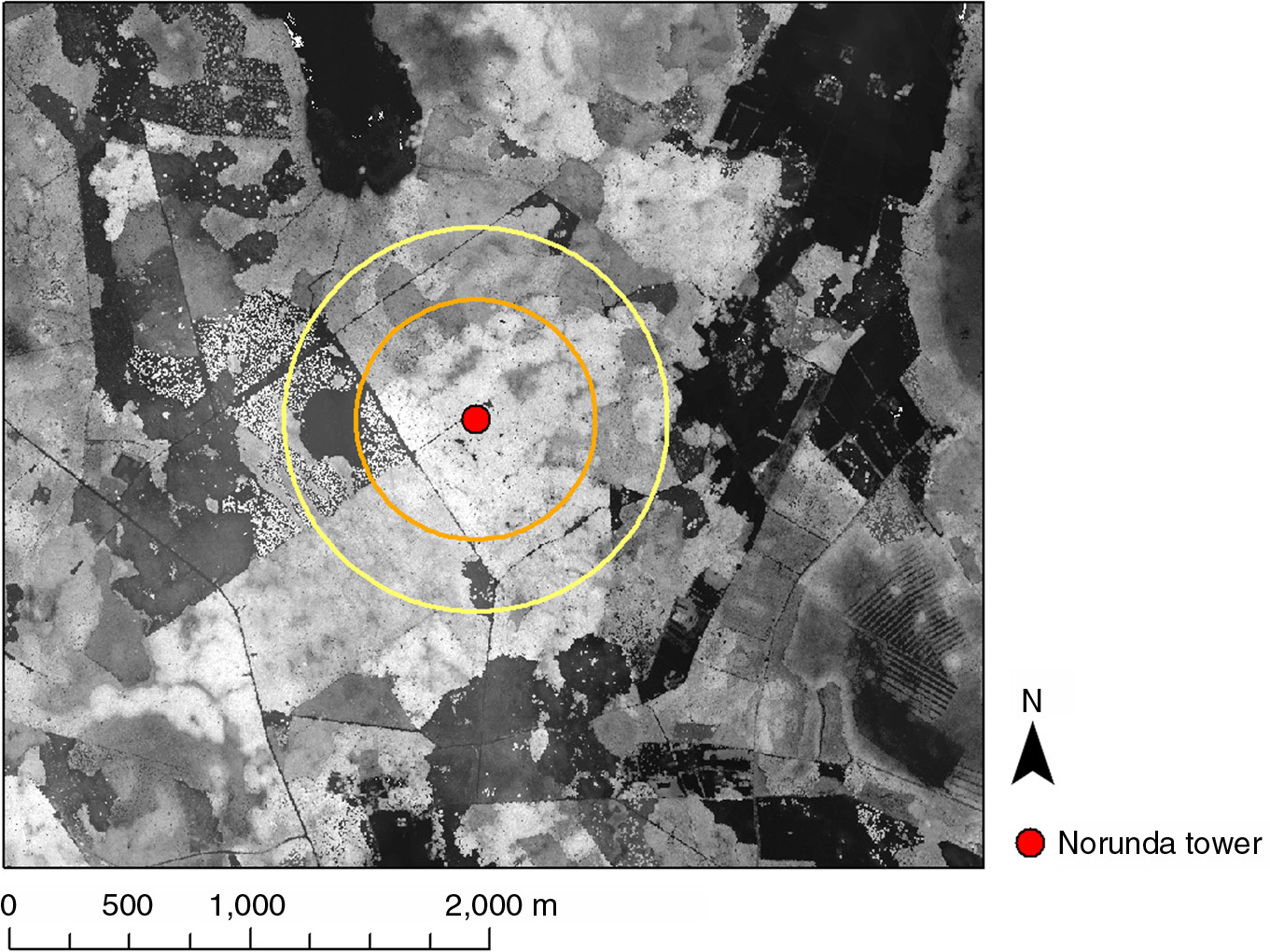
Fig. 1
Digital surface model (DSM) of the Norunda site. The circles denote 500 m (orange) and 800 m (yellow) distance from the tower (red dot).
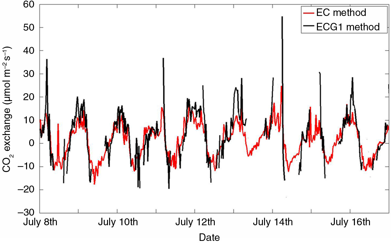
Fig. 2
Comparison of net CO2 exchange measured by EC at 33 m and net CO2 exchange calculated from gradients between 31.7 and 58.8 m by combined EC and gradient method (ECG) in July 2010. For the ECG method, only values with good accuracy, i.e., total errors <20 µmol m−2 h−1, are shown (see text for details).
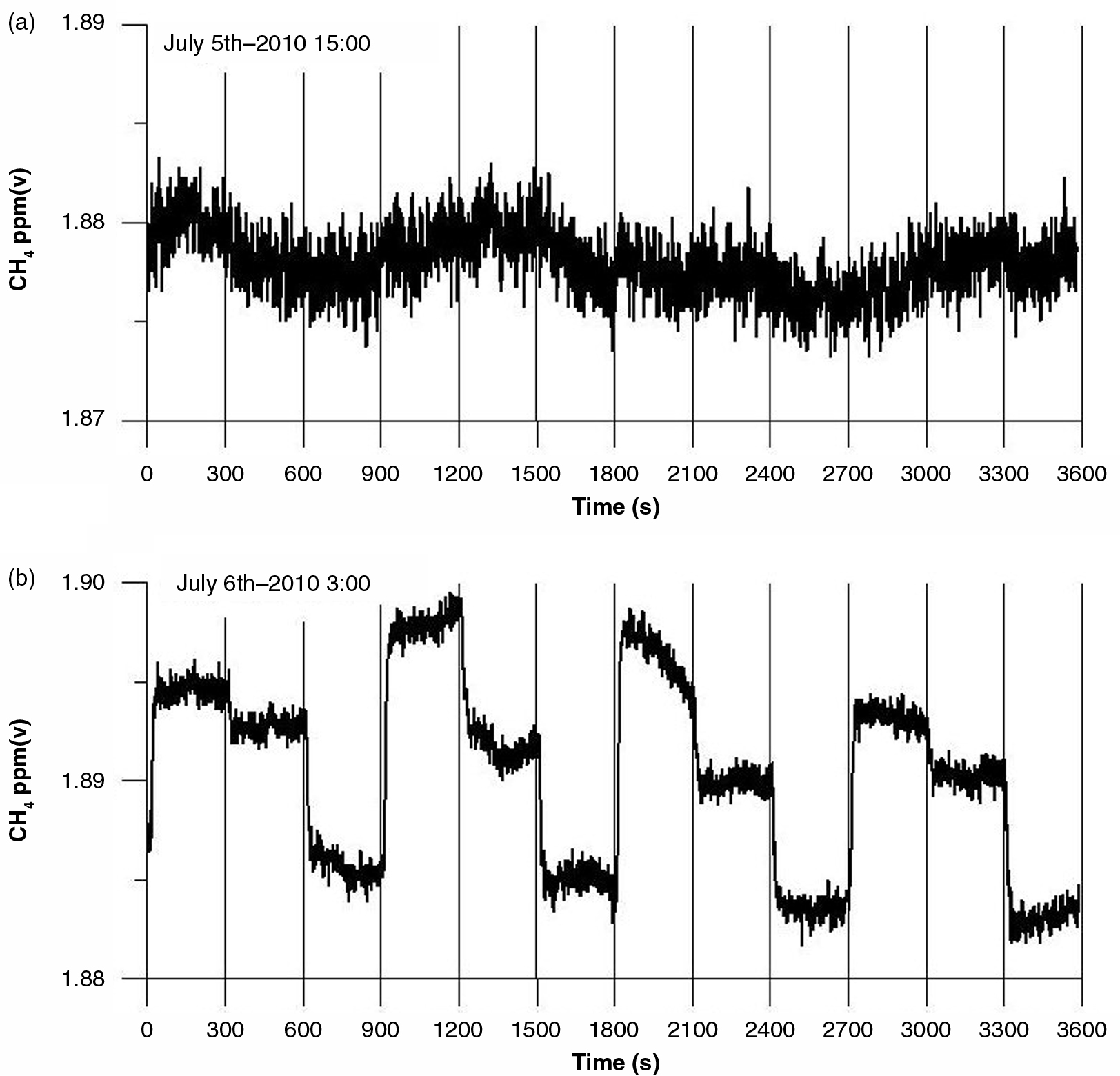
Fig. 3
Example of (a) daytime and (b) nighttime CH4 concentration measurements. Each level (31.7, 58.8 and 100.6 m) was measured for 5 min=300 s starting at level 1.
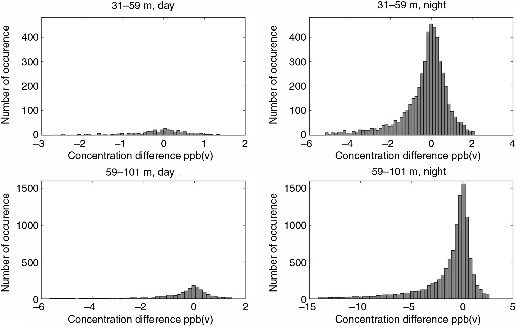
Fig. 4
Occurrence of CH4 concentration differences for different height intervals and for day (global radiation >50 Wm−2) and night (global radiation <50 Wm−2). Data between the 2nd and 98th percentiles are shown.
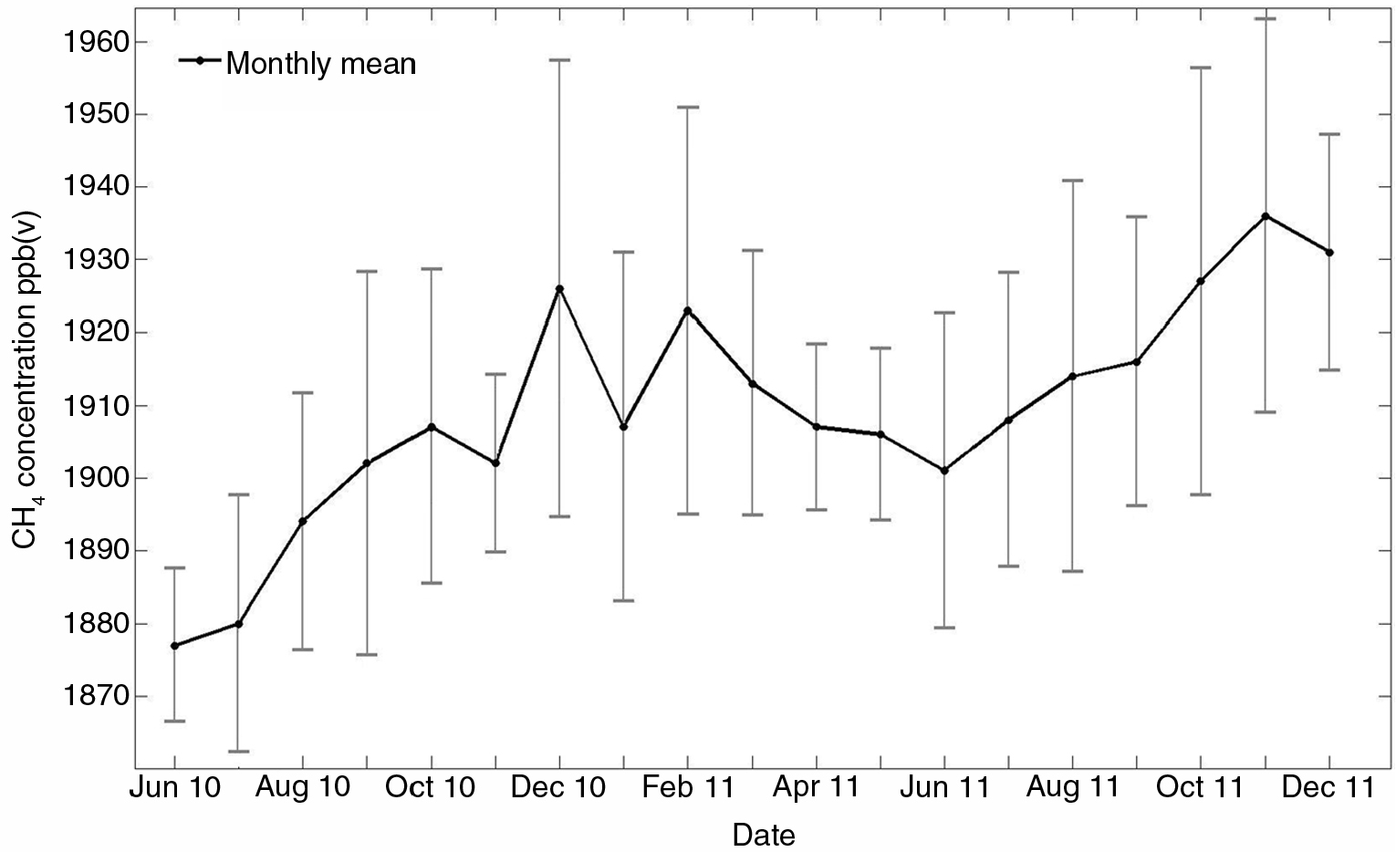
Fig. 5
CH4 concentration measured at 100.6 m height from June 2010 to December 2011. Error bars are given as plus/minus SD of monthly mean concentrations.
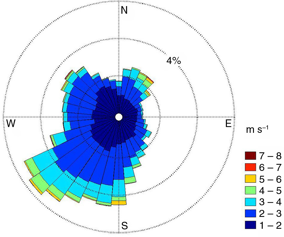
Fig. 6
Windrose for Norunda site at 33 m height above ground for the entire measurement period.
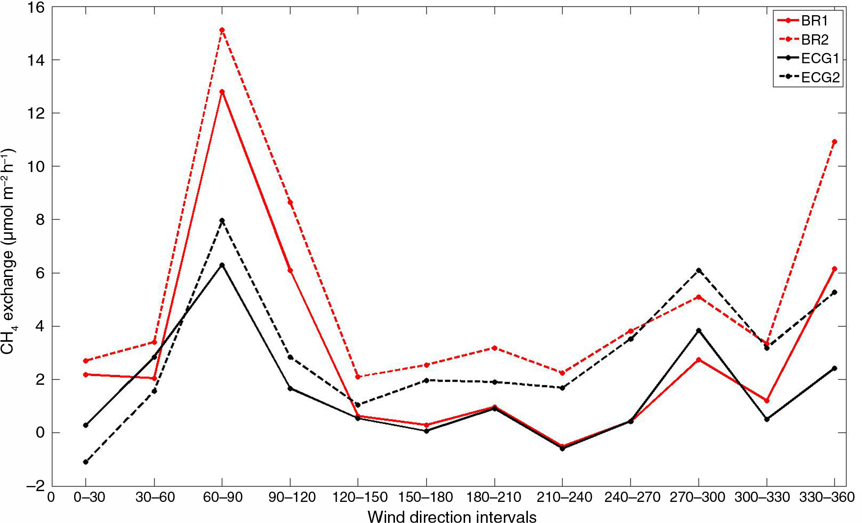
Fig. 7
Average CH4 exchange at the tower for wind directions binned in 30 degree intervals.
Table 1. Monthly mean values of CH4 exchange for main wind directions, 180°–240°, derived using the modified Bowen ratio (BR) method and the combined eddy covariance and gradient method (ECG) for gradients between 31.7 and 58.5 m and between 31.7 m and 100.6 m
CH4 exchange (µmol m−2 h−1)BR2
CH4 exchange (µmol m−2 h−1)ECG1
CH4 exchange (µmol m−2 h−1)ECG2
CH4 exchange (µmol m−2 h−1)Chambers
CH4 exchange (µmol m−2 h−1)Jun 20107.58.74.08.0–Jul 20101.955.61.2*3.8−11.7Aug 2010−1.72.1−2.72.4−9.8Sep20103.95.92.55.9−9.0Oct 20102.75.34.15.5–Nov20100.7*2.8−0.7*3.0–Dec2010−1.61.7*−1.91.1*–Mar 20110.3*3.51.02.2–Apr 20113.13.95.96.6–May 2011−0.3*1.7−1.4*1.2–Jun 20110.2*5.21.1*3.9–Jul 2011−1.2*1.3*−1.2*0.1*–Aug 2011−4.01.1*−3.71.8–Sept2011−2.71.1*−1.6*0.4*–Oct 20110.3*0.9*0.1*0.2*–Nov 2011−1.1−0.1*−1.4−1.4–Dec 2011−1.40.4*−3.1−0.4*–
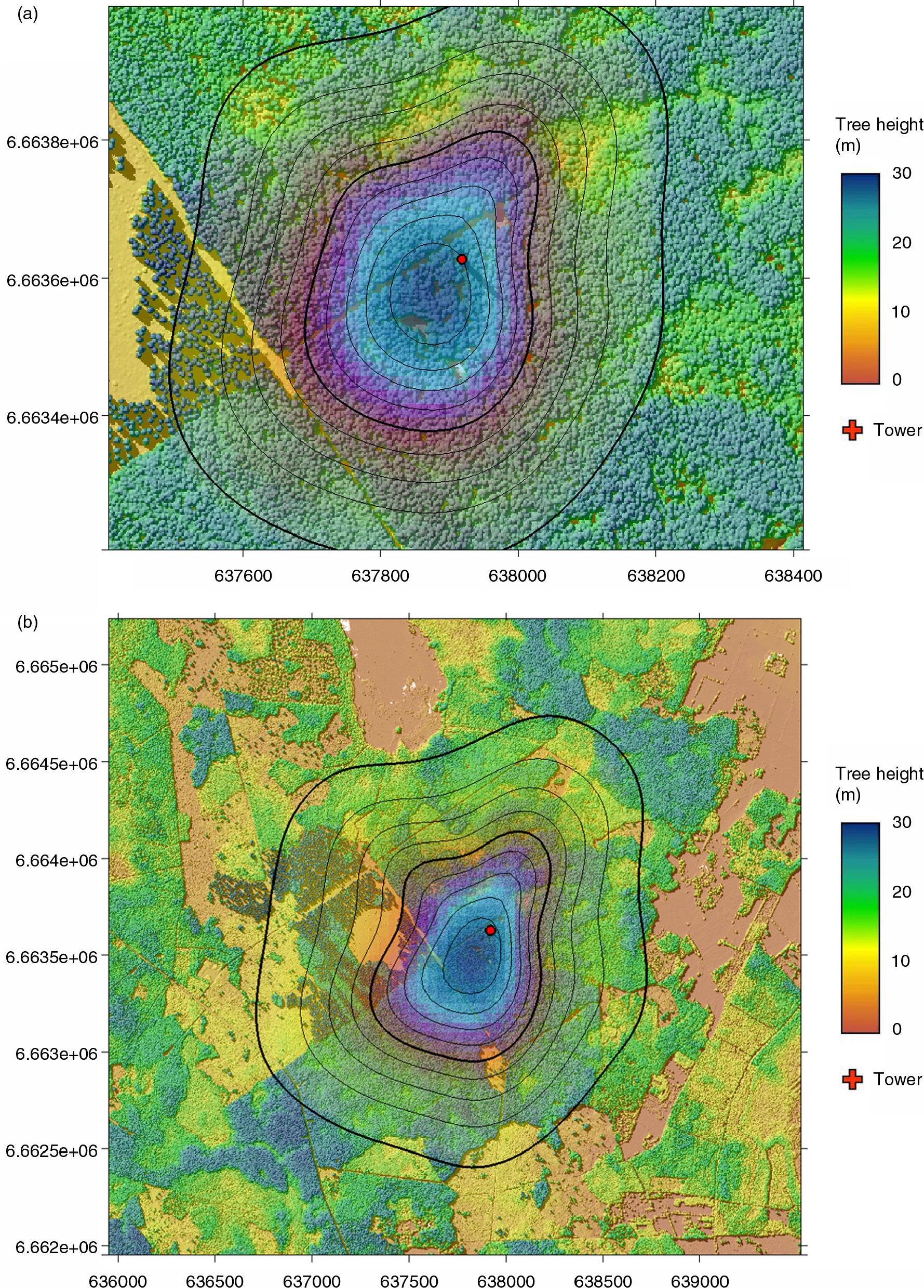
Fig. 8
Half-hourly footprint estimates cumulated for the entire measurement period for (a) gradients between 31.7 and 58.5 m and (b) between 31.7 and 100.6 m. Contour lines are plotted for each 10% of the cumulated footprint. The tower location is depicted as a red dot. The background maps are tree height from LiDAR measurements, for illustration. Coordinates (x and y axes) are in UTM.
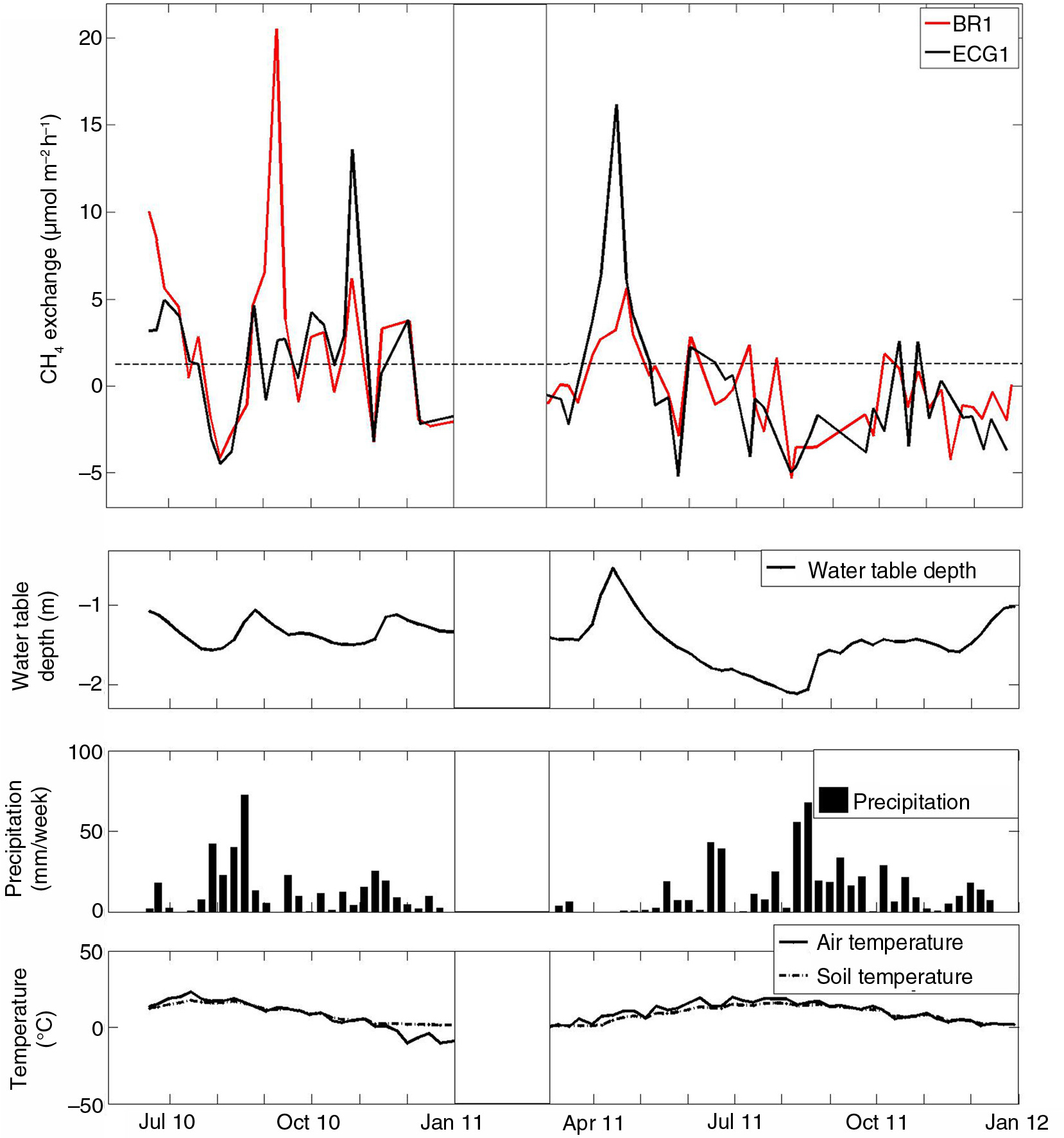
Fig. 9
Weekly mean values of CH4 exchange, water table depths, air temperature and soil temperature and also the weekly amount of precipitation.
Table 2. Coefficients calculated by multiple linear regression analyses of daily mean values of CH4 exchange derived at two levels and for two different methods (the modified Bowen ratio (BR) method and combined eddy covariance and gradient method (ECG)); and the explanatory variables air temperature, soil temperature, soil moisture, water table depth, CO2 exchange and GPP. The analysis was made on standardised data to adjust for the disparity in variable sample sizes. The adjusted R 2 value displays how much of the variance in CH4 exchange can be explained
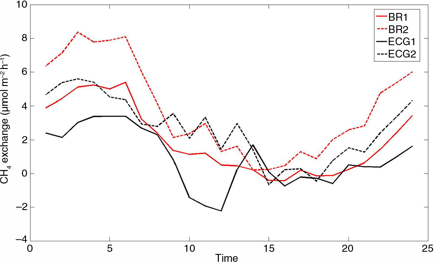
Fig. 10
Diel pattern of CH4 exchange binned hourly for the entire measurement period.
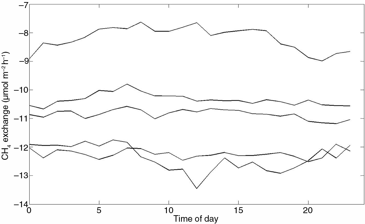
Fig. 11
Diel patterns of soil CH4 exchange measured by individual soil chambers, 7 July–31 September 2010.
Table 3. Pearson correlations between hourly binned CH4 exchange for BR1 and hourly binned air temperature, soil temperature, GPP and VPD