Have a personal or library account? Click to login
Spatio-temporal variation of total mercury in precipitation in the largest industrial base in China: impacts of meteorological factors and anthropogenic activities Cover

Spatio-temporal variation of total mercury in precipitation in the largest industrial base in China: impacts of meteorological factors and anthropogenic activities

Open Access
|Jan 2015

Figures & Tables

Fig. 1

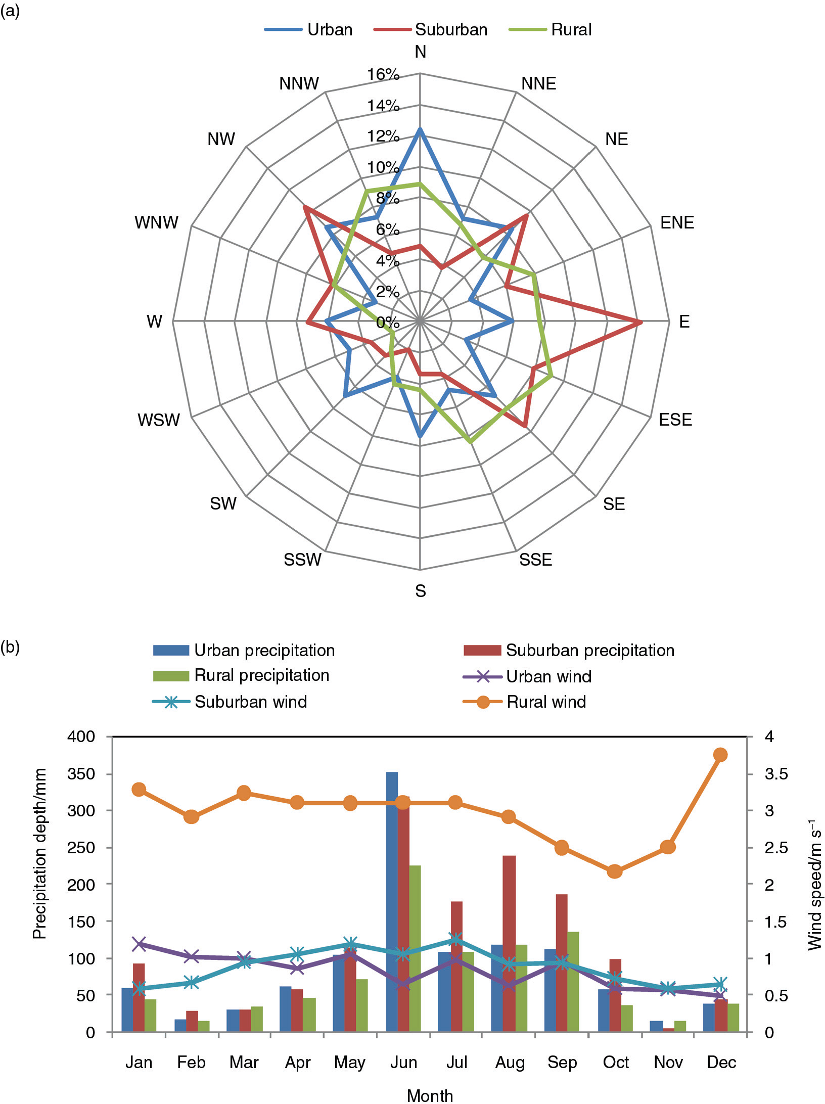
Summary statistics of the meteorological data at urban, suburban and rural sampling sites. The wind rose diagrams are shown in (a), and (b) illustrates monthly precipitation depth and wind speed.
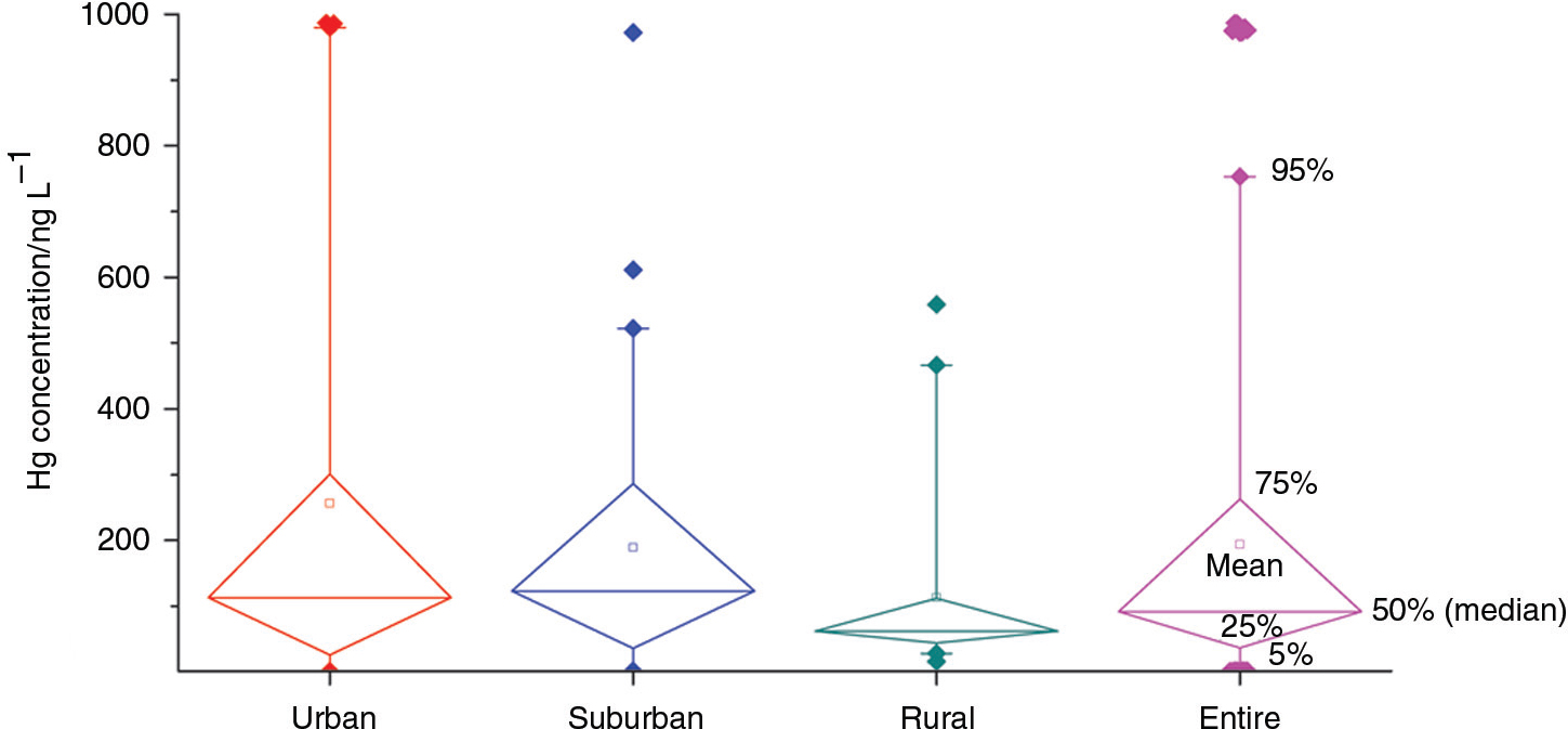
Fig. 2

Summary statistics of Hg concentrations in precipitation collected at urban, suburban and rural sites.

Table 1. Comparison of total Hg concentrations in precipitation in different regions/ng L−1
RegionAverage/rangeSampling periodSourceUrban site, Shanghai, China113a/1–987b2008–2009This studySuburban site, Shanghai, China122a/2–973b2008–2009This studyRural site, Shanghai, China62a/16–559b2008–2009This studyBeijing, China277–1139b1995 Liu et al. (2000)Changchun (heating season), China405/150–718b1999–2000 Fang et al. (2004)Changchun (non-heating season), China235b1999–2000 Fang et al. (2004)Wujiang River Basin, China36/7.5–149b2006 Guo et al. (2008)Chongqing, China30.7/6.0–158b2010–2011Wang et al. (2012)Nam Co, China4.8/0.4–35b2009–2011Huang et al. (2012)Lhasa, Tibet, China24.8/3.1–178b2010Huang et al. (2013)Minnesota, USA170–3400b1982–1983 Glass et al. (1986)Great Lake Region, USA13.5/10–60b1997–2003 Hall et al. (2005)New York rural site, USA5.5b2004 Lai et al. (2007)Florida, USA10b1993–1996 Guentzel et al. (2001)Newcomb, NY, USA0.2–28b2004–2006 Choi et al. (2008)Underhill, Vermont, USA0.9–90.5b1995–2006 Gratz et al. (2009)Illinois, USA0.9–243.9b2007–2009Gratz et al. (2013)New Hampshire, USA1.4–65b2006–2009Lombard et al. (2011)Ahvaz city, Iran770b2011Ghadaksaz zadeh et al. (2014)Toronto, Canada22/29–37b2005–2006Zhang et al. (2012)Alberta, Canada2.1–67.7b2006–2008 Prestbo and Gay (2009)Sub-Arctic Alberta, Canada0. 3–27.8b2006–2008Sanei et al. (2010)Langenbrügge, Germany52b1992 Ebinghaus et al. (1999)Neuglobsow, Germany4.7–23.3b1998–1999 European Commission (2001)A rural wetland, France15/ < 15–20b2010–2012Connan et al. (2013)Sweden11.9/9.7–13.5b1991–1994 Munthe et al. (1995)Northern Europe4.2–19.8b1995–1999 European Commission (2001)Mace Head, Ireland4–12.2b1995 Ebinghaus et al. (1999)Lake Balaton, Hungary5.2–191b2000–2001 Nguyen et al. (2005)Town of Idrija, Slovenia3–24.4b2006–2007Kocman et al. (2011)NSW (urban), Australia1–19b2006–2007 Dutt et al. (2009)Tokyo (urban), Japan8.7c2002–2003 Sakata and Marumoto (2005)Hyogo (urban), Japan9.5c2002–2003 Sakata and Marumoto (2005)Hokkaido (rural), Japan8c2002–2003 Sakata and Marumoto (2005)Seoul (urban), Korea10–16.3b2006–2007Seo et al. (2012)Chuncheon (rural), Korea8.8b2006–2008Ahn et al. (2011)Pretoria, South Africa15.8/3.8–60.7b2007–2009Gichuki and Mason (2013)Cape Point, South Africa10.6/1.2–52.5b2007–2009Gichuki and Mason (2013)Olkaria, Kenya0.2–60b2009–2010Wetang'ula (2011)Amazon catchment, Brazil3.7–23.4b1996–1997 Fostier et al. (2000)Pengjiayu (remote islet), Taiwan8.5/2.3–22b2009Sheu and Lin (2013)Mt. Bamboo, Taiwan9.6/0.5–165.5b2009Sheu and Lin (2011)North Pacific Ocean14.3b2002 Laurier et al. (2003)Bermuda4.7b2008–2009Gichuki and Mason (2014)Equatorial Pacific Ocean2.9b1990 Mason et al. (1992)Indian Ocean0.9c2010–2011Shi et al. (2015)

[i] aThe median of Hg concentrations. The median can better depict the data set compared with the average, considering that a large variability in Hg concentrations exists (for details, see the main text).

[ii] bTotal Hg in bulk rain, including dissolved and particulate fractions of Hg.

[iii] cDissolved fraction of Hg.

Fig. 3

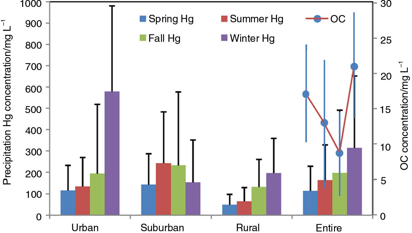
Seasonal variation of Hg and organic carbon (OC) in precipitation at urban, suburban and rural sampling sites. The four closed circles are OC concentrations in spring, summer, fall and winter. Error bars denote one standard deviation (1σ).
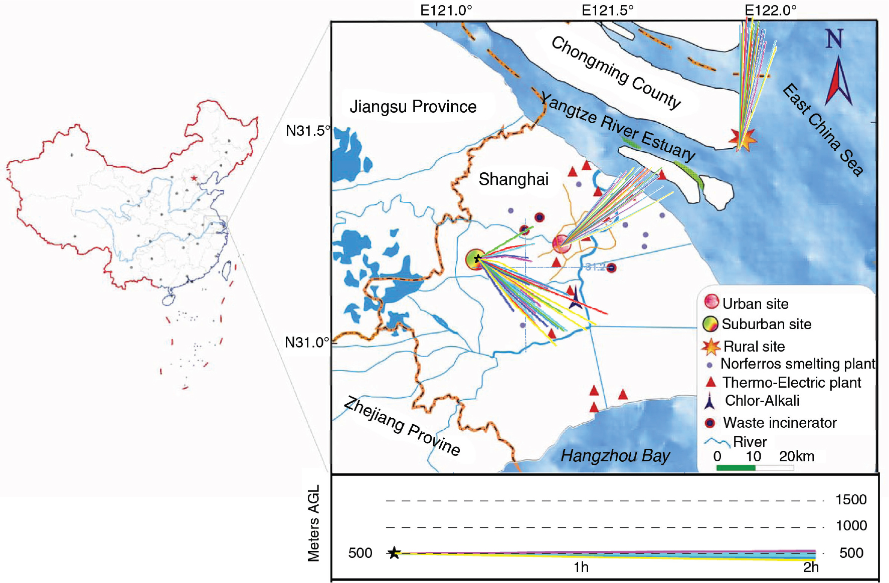
Fig. 4

The 2 h backward trajectories of precipitation events with high Hg levels at the three sampling sites, that is, 986, 973 and 559 ng L−1 for urban, suburban and rural precipitation, respectively. The end-point elevation of the trajectories is 500 m above ground level (AGL). The vertical velocity model was selected for the calculation of vertical motion.
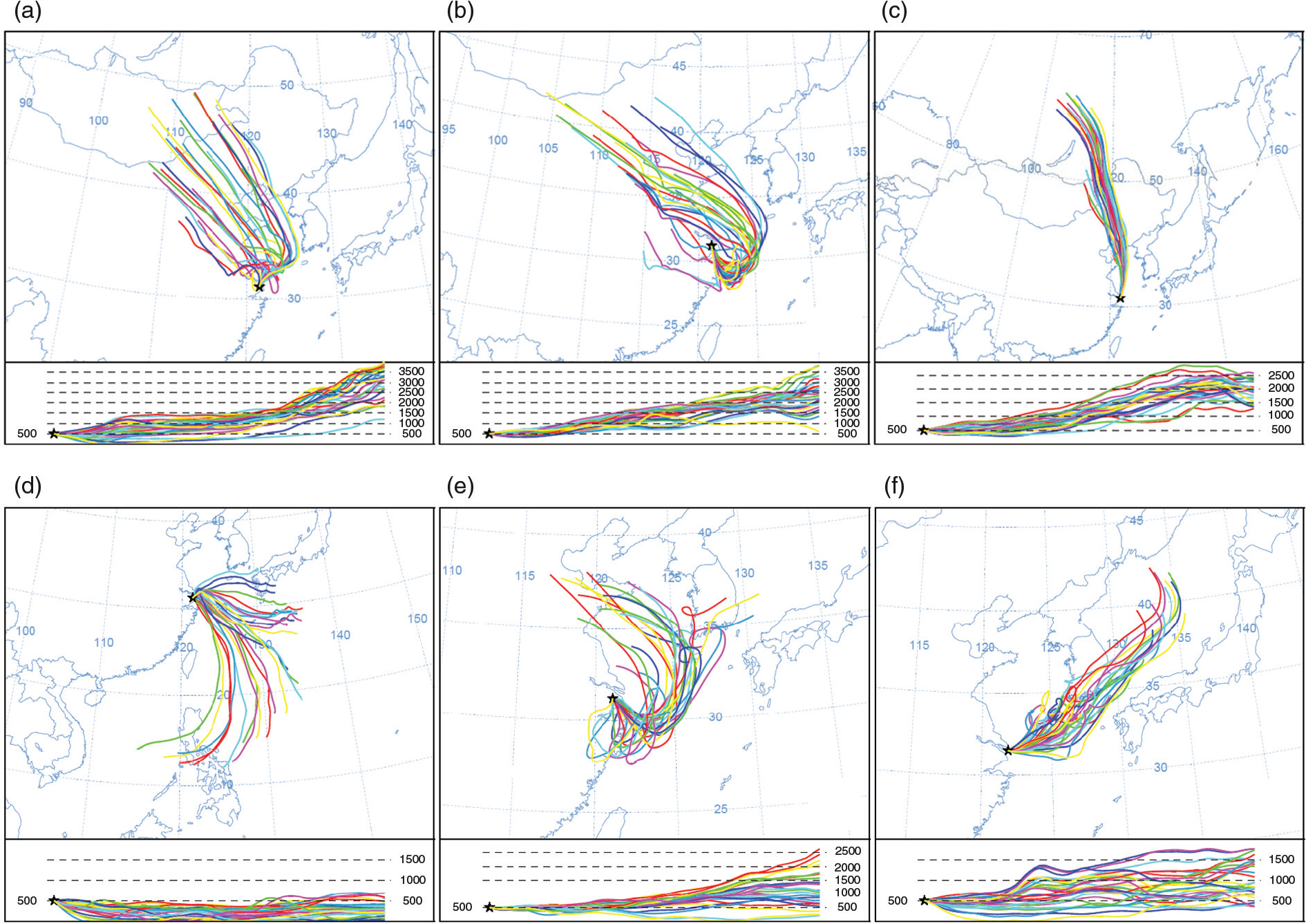
Fig. 5

The 72 h backward trajectories of precipitation events with higher and lower Hg levels at the three sampling sites. (a), (b) and (c) present the higher Hg concentration events at urban (987 ng L−1), suburban (610 ng L−1) and rural (559 ng L−1) sites, respectively; while figures (d), (e) and (f) are for the events with low Hg levels at urban (1 ng L−1), suburban (2 ng L−1) and rural sites (2 ng L−1), respectively. The method is the same as that of Fig. 4.

Language: English
Page range: 25660 - 25660
Submitted on: Aug 6, 2014
Accepted on: Jun 30, 2015
Published on: Jan 1, 2015
Published by: Stockholm University Press
In partnership with: Paradigm Publishing Services

© 2015 Guitao Shi, Zhenlou Chen, Jiyang Teng, Yuansheng Li, published by Stockholm University Press
This work is licensed under the Creative Commons Attribution 4.0 License.