
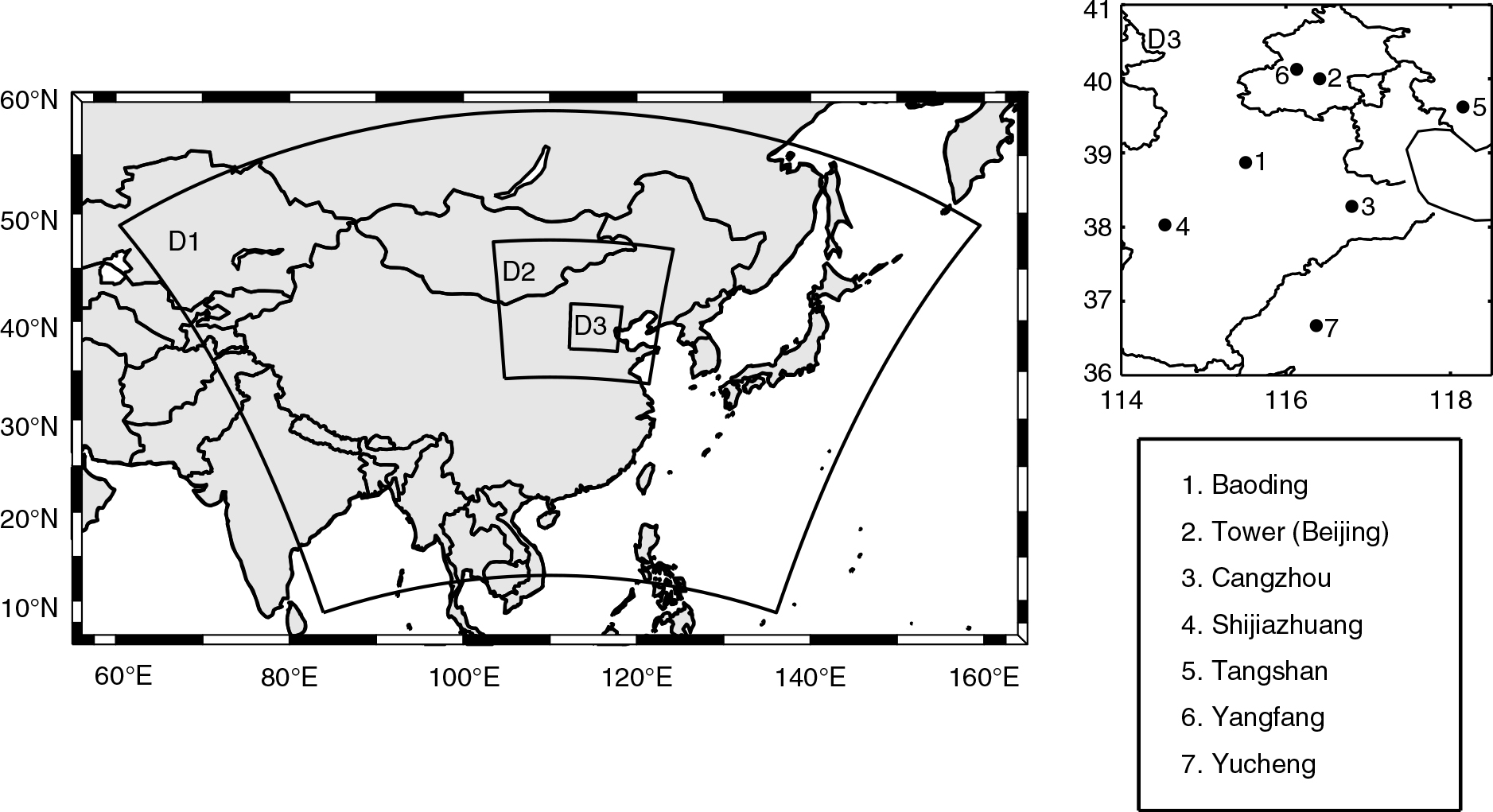
Fig. 1
Modelling domains and the monitoring sites over the BTH region.
Table 1. Design of WRF–Chem simulations to evaluate the effects of the additional HONO sources
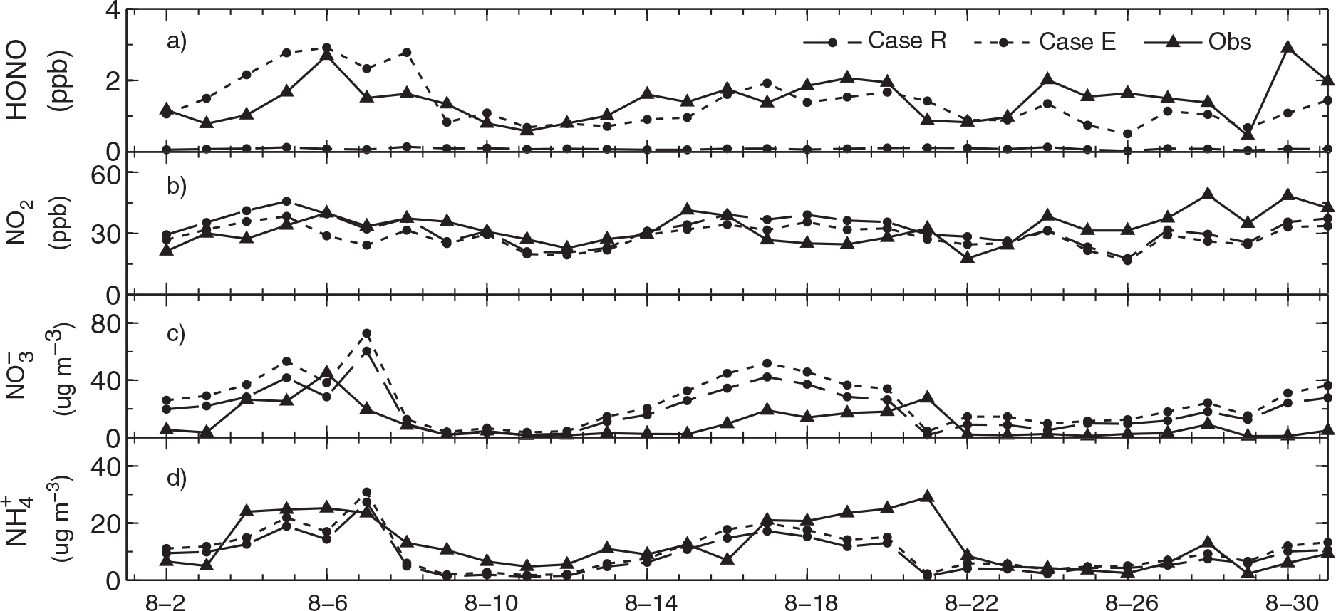
Fig. 2
Comparison of simulated 24-h average (a) HONO, (b) NO2, (c) and (d) concentrations with observations at Peking University during August 2007 (Ianniello et al., 2011; Spataro et al., 2013). Case R is a reference case; Case E includes the HONO emissions, NO2 * chemistry and NO2 heterogeneous reaction on aerosol surfaces.
Table 2. Statistics for comparison of the observed (Obs.) and simulated (Sim.) hourly data during August 13–20, 2007
[i] Observations of HONO are from the Beijing Meteorological Tower and the meteorological parameters are from the Olympic Village near to the tower site (see Section 3). NO2, O3 and PM2.5 measurements are from the seven urban sites over the BTH region (Fig. 1). Model results are for Case E.
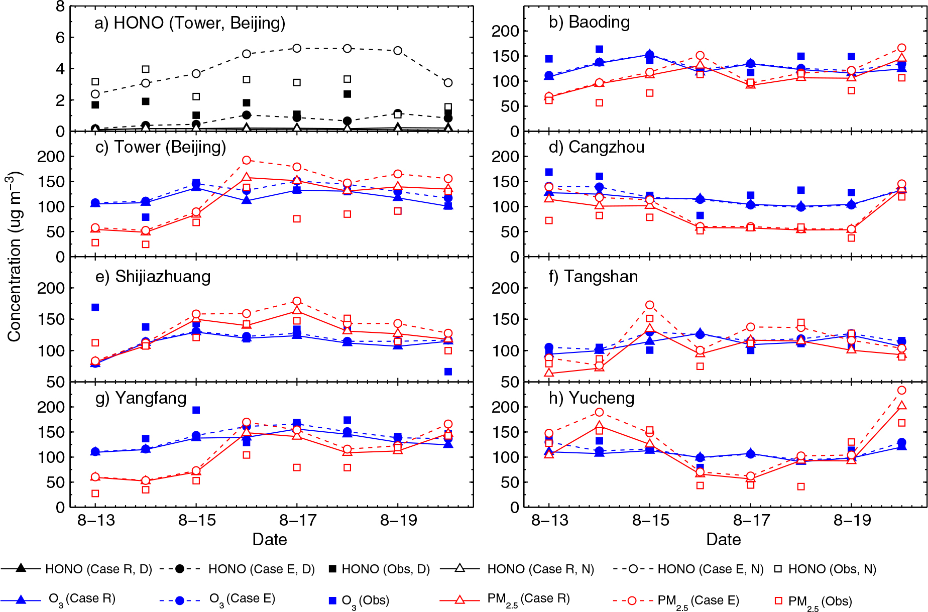
Fig. 3
Observed and simulated (a) daytime (D, 7:00–19:00) and night-time (N, 20:00–6:00) mean concentrations of HONO at the Beijing Meteorological Tower site and (b–h) daytime mean concentrations of O3 and PM2.5 at the seven urban sites over the BTH region during 13–20 August, 2007. The unit used is µg m−3 (at 1.01325×10⁵ Pa and 25°C, 1 µg m−3 is ~0.52 ppb for HONO and ~0.51 ppb for O3).
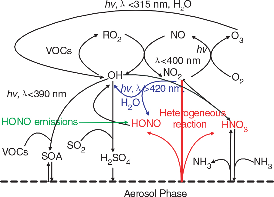
Fig. 4
Impacts of the additional HONO sources on the chemical coupling between ozone and particulate matter. HONO sources increase OH concentrations and subsequently promote O3 and PM production. HNO3 produced from the NO2 heterogeneous reaction on aerosol surfaces enhances nitrate concentrations in presence of NH3.
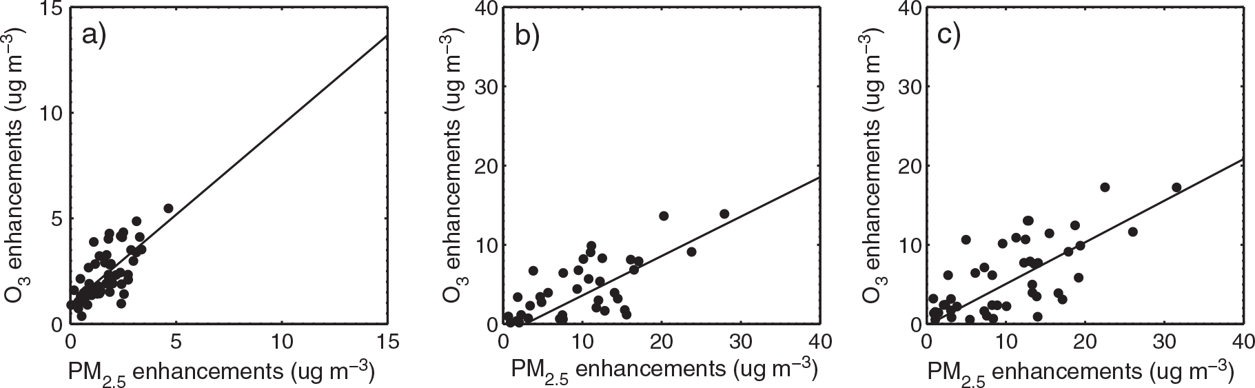
Fig. 5
Enhancements of daytime mean concentrations of O3 and PM2.5 due to (a) the NO2 * chemistry (b) the NO2 heterogeneous reaction on aerosols and (c) all the three additional HONO sources at the seven urban sites demonstrated in Fig. 3 during 13–20 August, 2007.
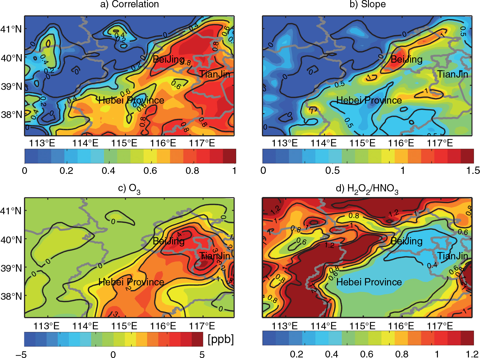
Fig. 6
Values of (a) the correlation coefficient and (b) the linear-fitting slope for O3 and PM2.5 daytime enhancements due to the three additional HONO sources during August 2007; monthly mean daytime (c) O3 enhancements due to the three additional HONO sources and (d) H2O2/HNO3 ratio over the BTH region.
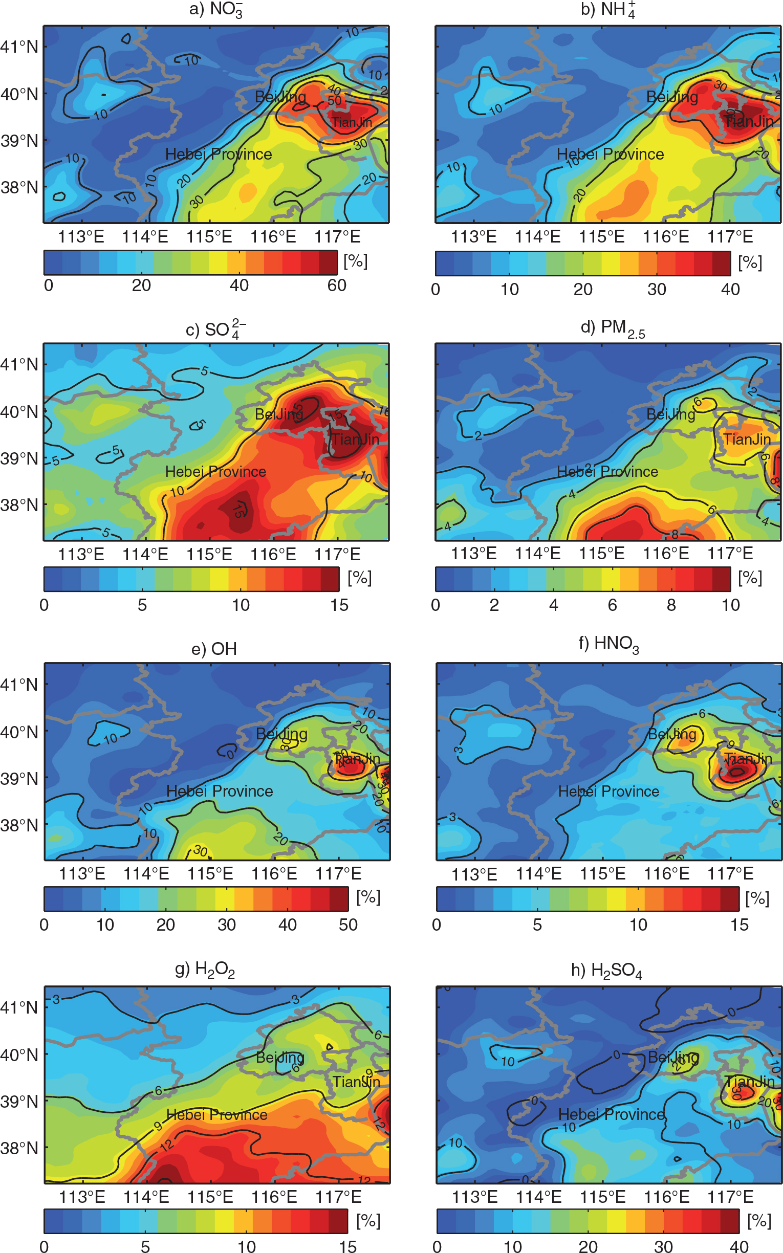
Fig. 7
Percentage increases of monthly-mean daytime (a) , (b) and (c) in PM2.5 and (d) PM2.5, (e) OH, (f) HNO3, (g) H2O2 and (h) H2SO4 concentrations over the BTH region during August 2007 due to the three additional HONO sources.
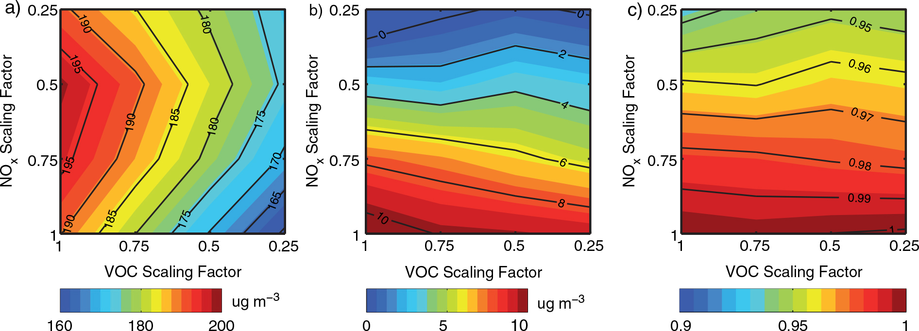
Fig. 8
Impacts of the additional HONO sources on O3_8h;max concentrations resulting from the control of NOx, VOC and NH3 emissions. (a) O3_8h;max concentrations for Case R in Beijing on 17 August 2007; (b) O3_8h;max concentrations for Case E minus those for Case R; (c) ratio of Relative Reduction Factors (RRF) for Case E divided by RRF for Case R.
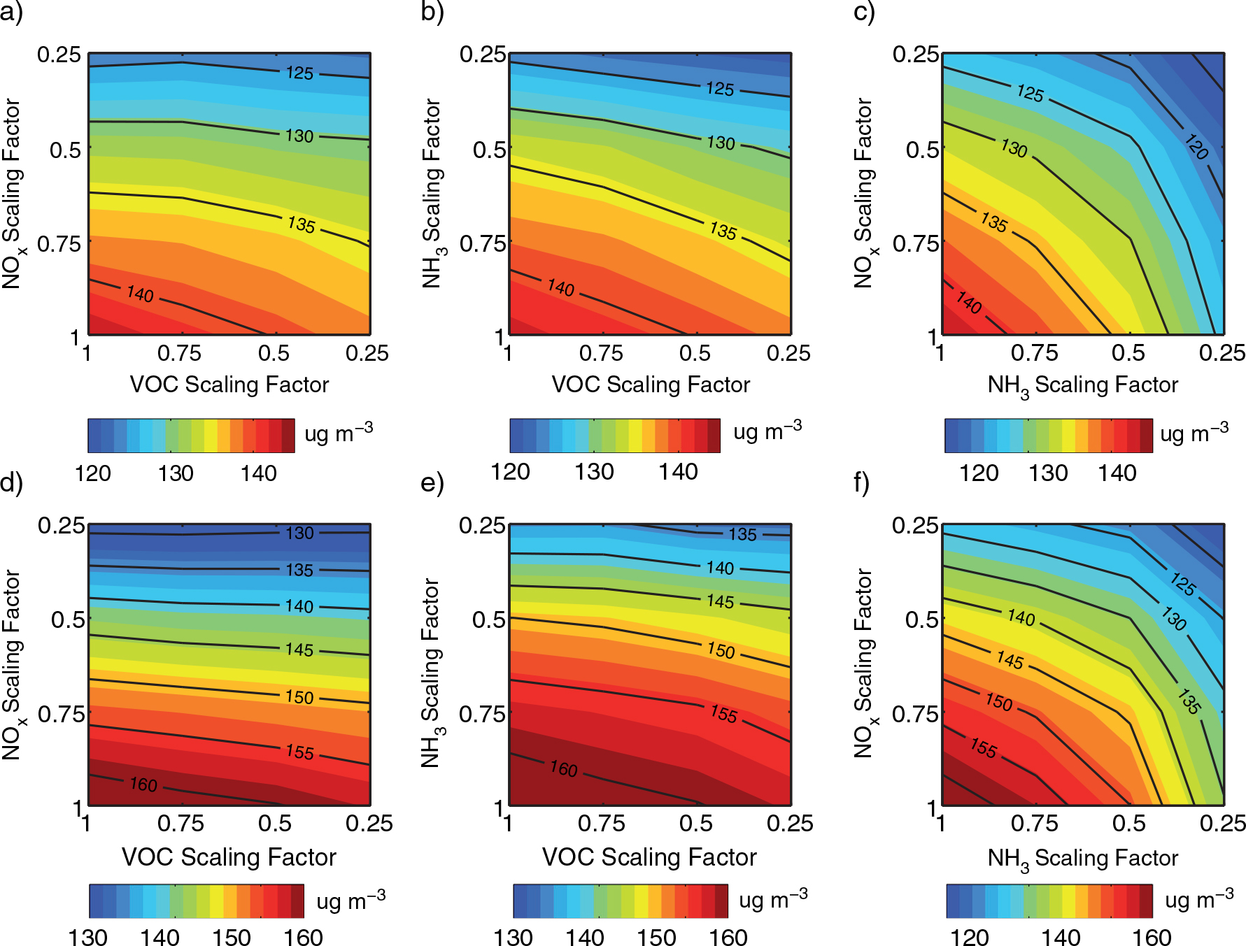
Fig. 9
Twenty four-hour average PM2.5 concentrations for Case R (a–c) and for Case E (d–f) in Beijing on 17 August 2007.
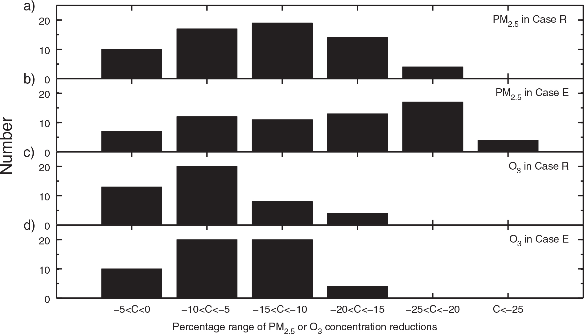
Fig. 10
The number of concentration reductions (C, with unit of %) of (a) PM2.5 in Case R, (b) PM2.5 in Case E, (c) O3 in Case R, and (d) O3 in Case E in a certain reduction range among the sensitivity simulations using the 64 emission scenarios (see Section 2.2).
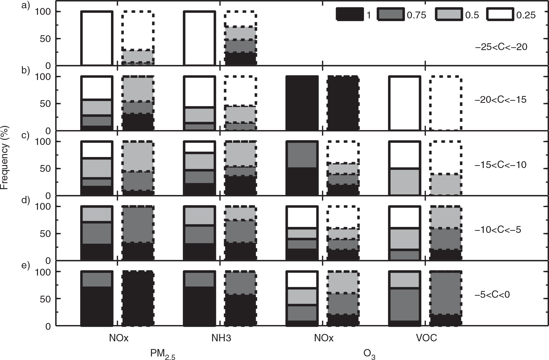
Fig. 11
Comparison of NOx, VOC and NH3 emission reductions between Case R (bars with solid baselines) and Case E (bars with dotted baselines) to gain the same range of PM2.5 or O3 concentration reductions (C, in unit of %) of (a) −25%<C<−20%; (b) −20%<C<−15%; (c) −15%<C< −10%; (d) −10%<C<−5%; and (e) −5%<C<0. The frequency for each scaling factor is computed by T i/T, where T is the total times for PM2.5 or O3 concentration reductions falling in a certain reduction range; T i is the occurrence times within T for a specific scaling factor (1, 0.75, 0.5 or 0.25 shown in Section 2.2).