
Fig. 1
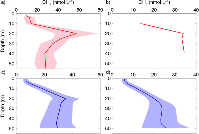
(a) Observed depth-profile of CH4 in the Laptev Sea in September 2007 from the PANGEA database, average (red line) and STD (pink area). (b) Observed depth-profile for one profile of CH4 in the Laptev Sea, September 2007, from the PANGEA database. (c) Modelled daily average of CH4 (blue line) with in situ production for July–September 2000–2009 and the STD (blue area). (d) The same as (c) but without in situ production. Note the different scales at the x axes.
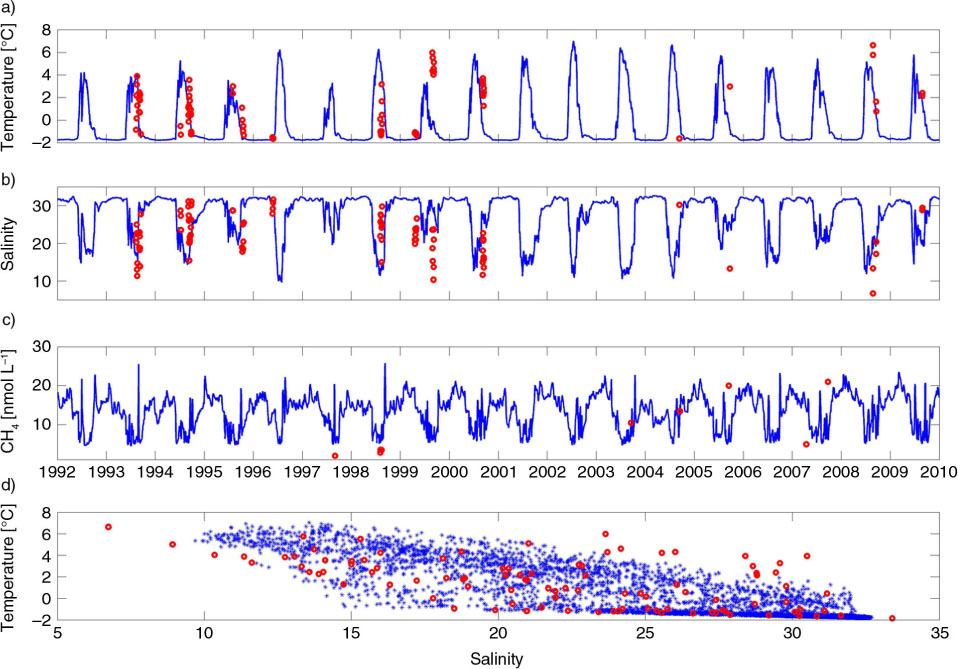
Fig. 2
Observed (red dots) and modelled surface values (blue solid line) of (a) temperature, (b) salinity, and (c) concentration of CH4 as function of time and (d) temperature–salinity diagram. Observations for (a), (b) and (d) are horizontal averages over the depth interval 4–5 m in the area between 115 to 135°E and 74 to 77°N. In panel (c), observations are estimated from the literature, see text.
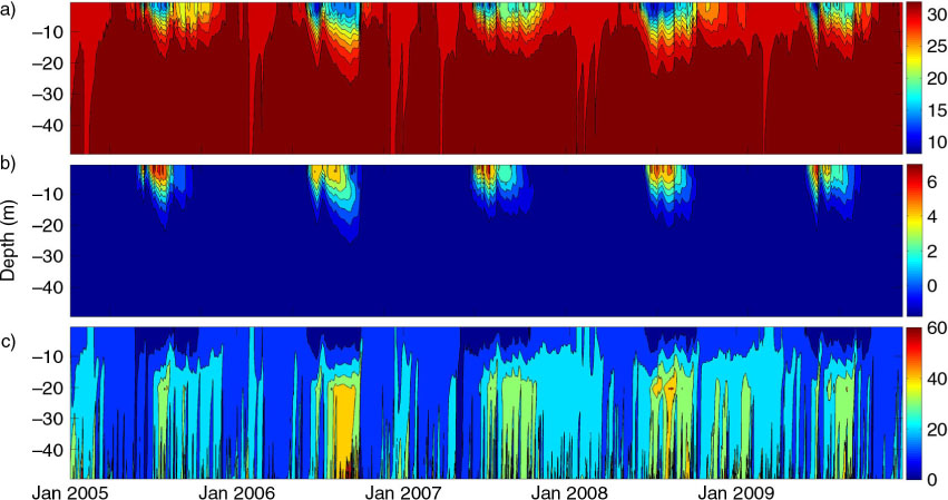
Fig. 3
Modelled time-series for the years 2005–2009: (a) salinity, (b) temperature and (c) concentration of CH4 as function of depth and time.
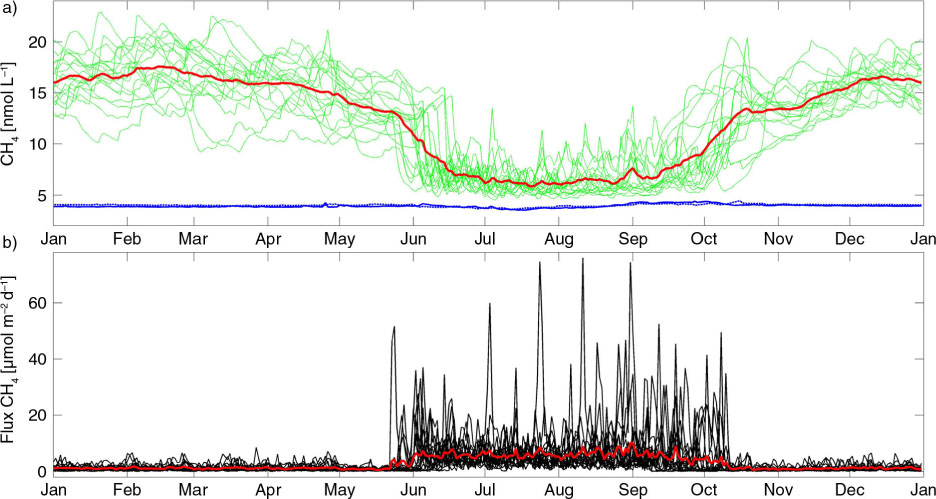
Fig. 4
(a) Daily mean simulated concentration of CH4 in the surface layer for the 18-yr (1992–2009) model simulation with present drivers (green line) and the average for the same period (red line). Included are the atmospheric pCH4 dissolved in seawater for 1992 (blue solid line) and 2009 (blue dotted line) at Point Barrow, Alaska. (b) The corresponding model output of sea–air exchange of CH4 for the same period (black lines), with the average value shown by the red line. Positive values denote fluxes from the sea to the air.
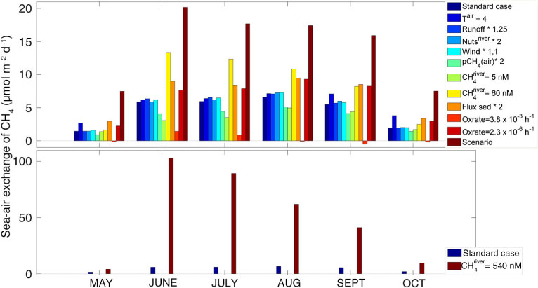
Fig. 5
Modelled monthly average net sea–air exchange for CH4 from May to October for the 18-yr (1992–2009) model run with different drivers. Standard case is dark blue in both upper and lower panel. Abbreviation to the right stands for: increased air temperature (Tair+4), increased river discharge (Runoff), nutrients in the river (Nutsriver), wind (Wind), CH4 in the atmosphere [pCH4(air)], increased concentration of CH4 in river runoff (CH4 river), flux from the sediment (Flux sed), oxidation rate in the water column (Oxrate) and the ‘worst case scenario’ (scenario). Note the different scales at the y-axes.
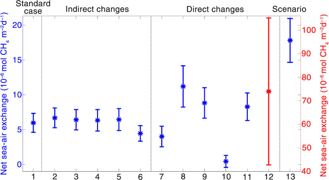
Fig. 6
Modelled annual average net sea–air exchange (star) and STD (bars) over 18 yr (1992–2009) for the ice-free period for the different experiments. The different simulations are also listed in Table 1 with numbers. Note the two y-axes.
Table 1. Modelled average net seasonal (ice-free period) and annual average net sea–air exchange over 18 yr (1992–2009) for different scenarios
[i] The results are grouped in scenarios with ‘indirect’ and ‘direct’ changes. The annual average net sea–air exchange is calculated for the Laptev Sea with an area of 498 000 km2 (Jakobsson, 2002). The bold numbers in column 3 are statistically significant at the 95% significance level, and blue numbers refer to decreasing values compared with the standard case.