
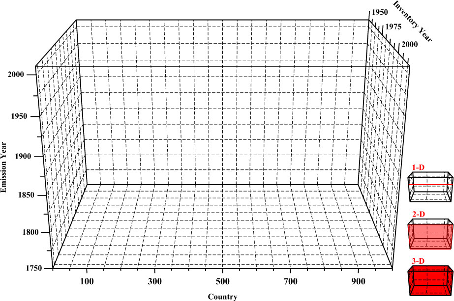
Fig. 1
The FFCO2 emissions estimate data cube. Countries along the x-axis could be labelled by name or number. Emission years used in this analysis range from 1950 to 2010. Inventory years used in the analysis range from 1984 to 2012. Each new release of the CDIAC FFCO2 inventory adds a new face to the data cube, displacing the old face toward the rear. Not all elements in the data cube are necessarily occupied by valid data. For example, country number 461 could represent Sabah which only has FFCO2 estimates for emission years 1950–1969. Data elements, for other emission years for this country regardless of the inventory year, are empty since this political unit did not exist in these other emission years. The cube could be filled with emission estimates based on production data only [using eq. (1)] or with emission estimates based on consumption data [additionally using eq. (2)]. The global total FFCO2 emissions for one emission year in one inventory year could be represented by a horizontal line on the face of the data cube (i.e. the sum of countries). If the cube is filled by consumption data, the global total would require an additional term for emissions that are not included in national totals (e.g. bunker fuels, Andres et al., 2012). For the latest release of the database, more than 107 000 elements of the production data cube are filled and more than 179 000 elements of the consumption data cube are filled. The three insets show which portion of the data cube are used for the 1-D, 2-D and 3-D cases.
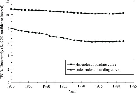
Fig. 2
The bounding uncertainty curves calculated for the 1-D case as would have been originally calculated by Marland and Rotty (1984). Each data point in each line is the result of the 1-D analysis. Values in the dependent bounding curve were calculated from ∑(f i *combinedi) and values in the independent bounding curves were calculated from √∑(f i *combinedi)2, where i=solid fuels, liquid fuels, gas fuels, gas flaring and cement; f is the fraction of the global source in a given year, and combined is from the Table 1 values. Note the 90% confidence interval (1.64 σ) is different than the 2 σ uncertainty assessment used throughout the rest of this manuscript.
Table 1. Uncertainty data pertinent to the 1-D case
[i] All values shown are at the 2 σ confidence interval and are shown to two significant digits only. Underlined values have been changed since the Marland and Rotty (1984) calculation. The solid CC uncertainty is new and is based on data reported in Marland et al. (1995), with a fixed coal: lignite ratio of 84: 16 informed by statistics from the entire 1950 to 2010 time series, n=2126. The liquid CC uncertainty is new and is based on data reported by Mash et al. (1995), n=29. The gas CC uncertainty is new and is based on data reported by Liss et al. (1992), n>6800. The gas flaring CC uncertainty is as reported in Boden et al. (1995). Cement uncertainties are discussed in the text. The combined column is the square root of the sum of the squares of FC, FO and CC and indicates the uncertainty for each source. Values shown below are held constant for all years. n=number of samples.
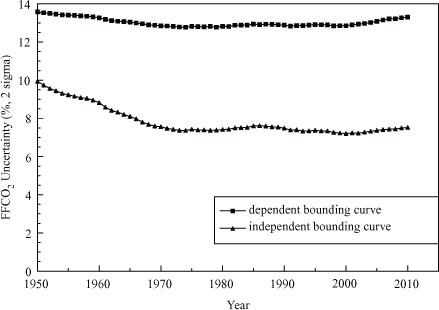
Fig. 3
The bounding uncertainty curves calculated for the 1-D case with all CC updates, cement uncertainties, and at 2 σ uncertainty. The true uncertainty value presumably lies between these bounding curves. Each data point in each line is the result of the 1-D analysis. Note the change in scales from Fig. 2 for both axes to accommodate increased uncertainty magnitude and additional years.
Table 2. Uncertainty values pertinent to the 2-D case
[i] As discussed in the text, these values are applied for all years. The largest FFCO2 emitter listed for each class is based on FFCO2 emission estimates for emission year 1990, the latest emission year available when the classes were first defined. The top emitters in each class are largely the same today with the latest inventory and emission year data, except that class 5 is now led by Russia which is only one of the current national entities that composed the former USSR.
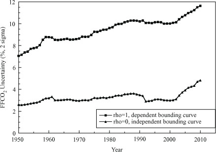
Fig. 4
The bounding uncertainty curves calculated for the 2-D case. Two-sigma uncertainty assessments are calculated for emission years 1950–2010. A better model of uncertainty lies between the two curves shown.
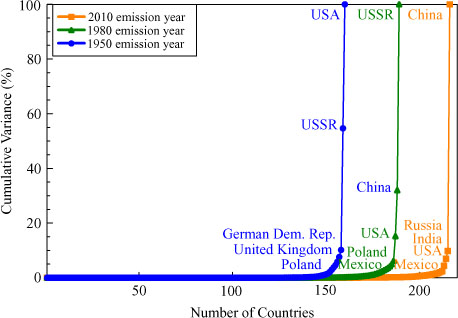
Fig. 5
The cumulative variance versus number of nations curve shows the contribution of each nation to total uncertainty. The top five FFCO2 emitting nations in each emission year are labelled. Some labels could not be clearly placed next to their adjacent data points, but are in the correct top to bottom order. Not all years have the same number of nations. Most nations contribute little to the total variance. All data are from the latest available inventory year.
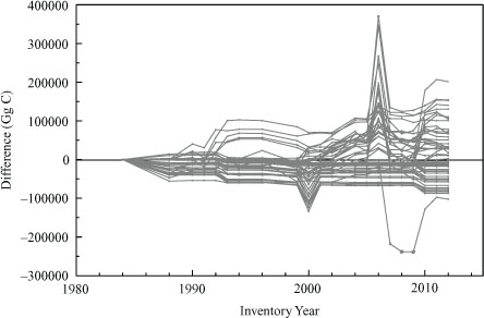
Fig. 6
3-D case: The difference in global FFCO2 emission estimates as calculated in subsequent inventory years for a given emission year. All curves start at zero by definition. The 61 individual emission years (i.e. 1950–2010) are not individually labelled. The first curve starting at the left of the plot is for emission year 1950 and shows the difference in reported 1950 emissions with each successive reported inventory (i.e. inventory years). Many emission years show an increase in the difference at inventory year 2006 which is discussed in the text.
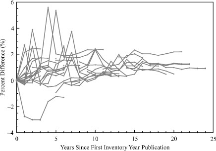
Fig. 7
3-D case: The per cent difference in global FFCO2 emission estimates as calculated in subsequent inventory years for a given emission year. All curves start at zero by definition. The 25 individual emission years are not individually labelled.
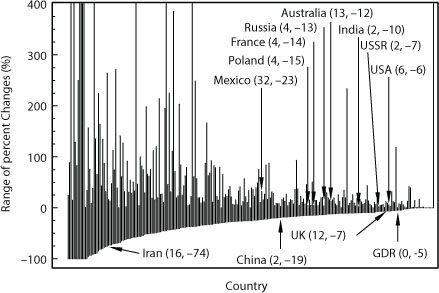
Fig. 8
Maximum and minimum range of per cent change in national emissions for a given emission year. Countries arranged by minimum changes. The group of countries at −100% are countries who had negative calculated emissions that were changed to near zero for this analysis. Eleven countries exceed 400% changes, from left to right (with maximum per cent in parentheses): Netherlands Antilles (2647), Congo (750), Somalia (14217), Gabon (1886), Cape Verde (540), United Arab Emirates (2952), Oman (2191), Côte d'Ivoire (734), Cook Islands (2714), Sierra Leone (2958) and Antarctic Fisheries (7176). Some countries are specifically labelled (with range in parentheses).
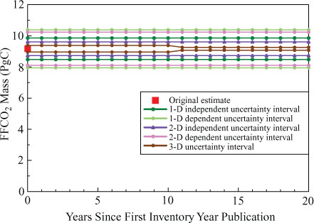
Fig. 9
Emission year 2010 global FFCO2 emissions with uncertainties explicitly shown based on the 1-D, 2-D and 3-D uncertainty cases. The time dependent 1-D and 2-D uncertainty cases plot as fixed values for this emission year.
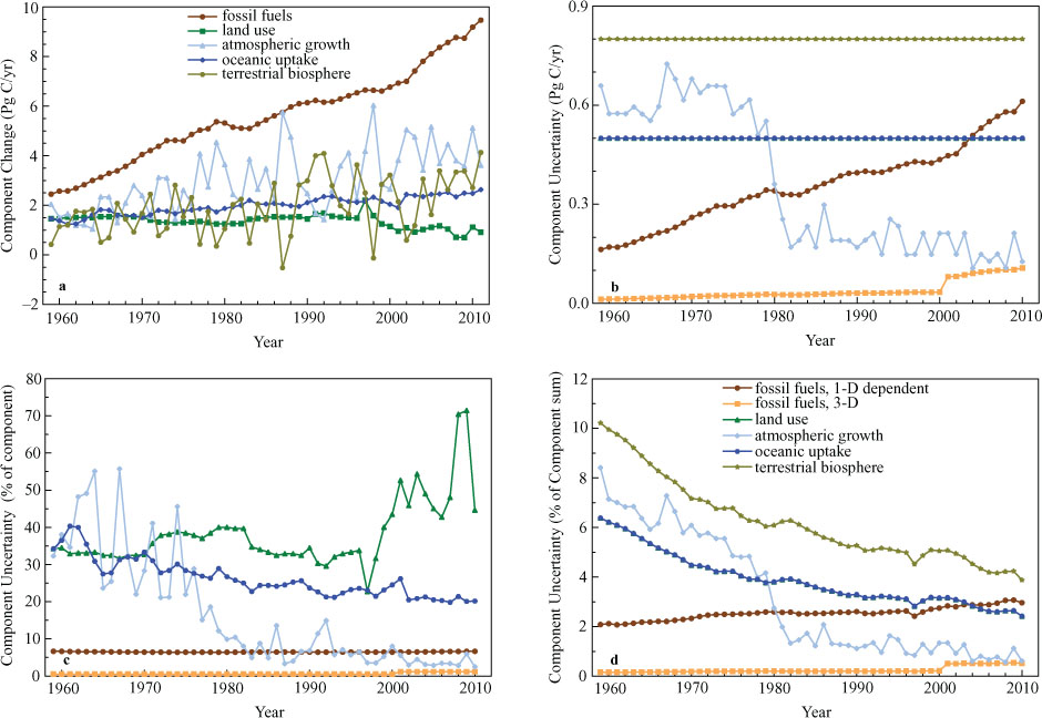
Fig. 10
FFCO2 compared to other global carbon cycle components. (a) GCP-reported mass flux and reservoir stock changes. Fossil fuels and land use change sources to the atmosphere are balanced by the sinks of atmospheric growth and oceanic uptake with the residual being accommodated by the terrestrial biosphere. (b) Component mass equivalent to 1 σ uncertainty. (c) One σ uncertainty, expressed in per cent of component mass. Terrestrial biosphere flux not shown as described in text. (d) One σ uncertainty, expressed in per cent of total carbon cycle flux and reservoir stock changes. Legend shown is applicable to panels b, c and d.