
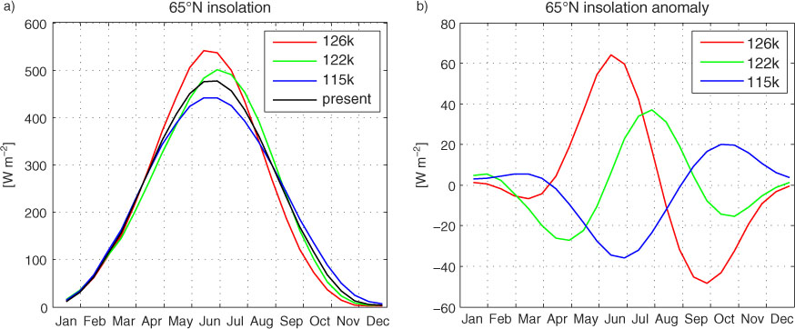
Fig. 1
(a) Monthly top of the atmosphere (TOA) shortwave radiation (SWR) [Wm−2] at 65°N for control run (ctrl), 115k, 122k and 126k calculated following Berger (1978). (b) TOA SWR anomalies at 65°N for Eemian time slices.
Table 1. Summary of boundary conditions for ECHAM4-iso simulations indicating source of sea surface temperature (SST), atmospheric CO2 [ppmv], CH4 [ppmv] and N2O [ppbv] concentration, eccentricity (Ecc.) [°], obliquity (Obl.) [°], precession (Pre.) [o(ω−180°)], glacier mask (Glac.) and vegetation mask (Vege.)
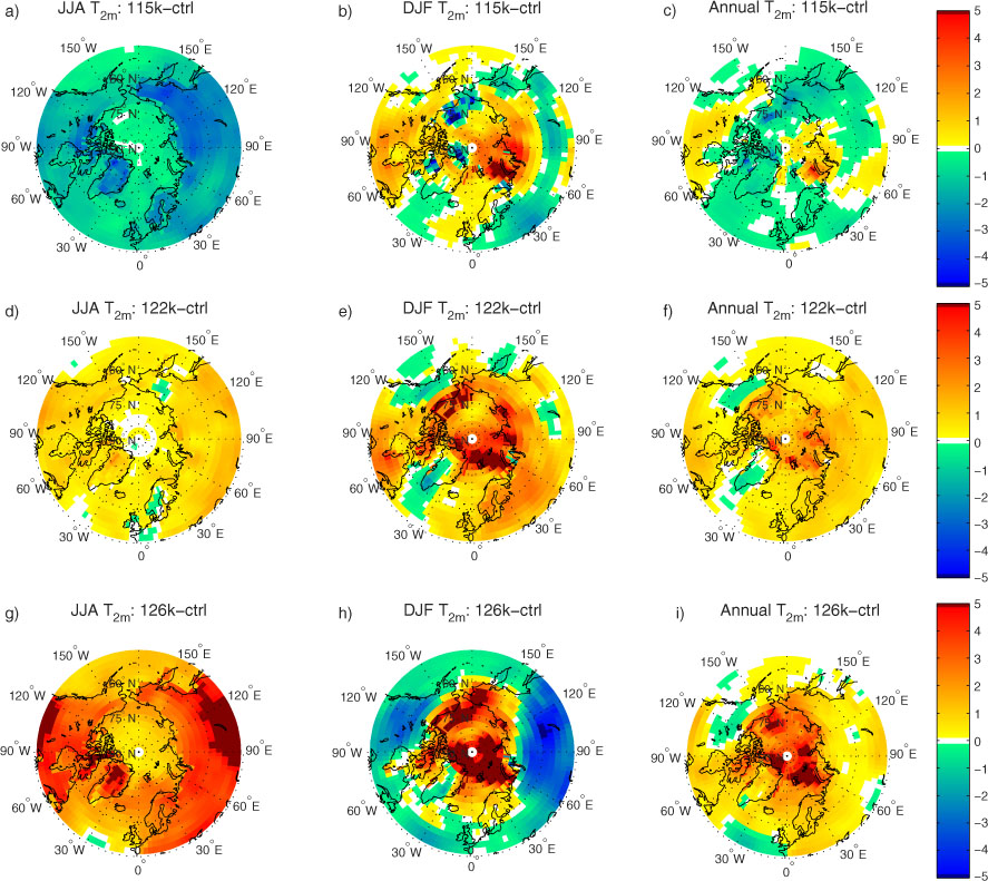
Fig. 2
Modelled JJA, DJF and annual mean 2m temperature (T2m ) anomalies north of 45°N for the 115k time slice (a) to (c), 122k time slice (d) to (f) and the 126k time slice (g) to (i).
Table 2. Absolute and anomalous GIS annual mean surface temperature [°C], annual mean precipitation weighted δ 18O [‰] and annual mean precipitation amount [mm/yr] above 1500 m for control run and Eemian time slices
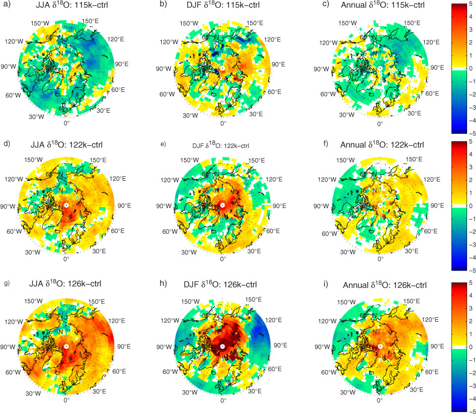
Fig. 3
Modelled JJA, DJF and annual mean precipitation weighted δ 18O anomalies north of 45°N for the 115k time slice (a) to (c), 122k time slice (d) to (f) and the 126k time slice (g) to (i).
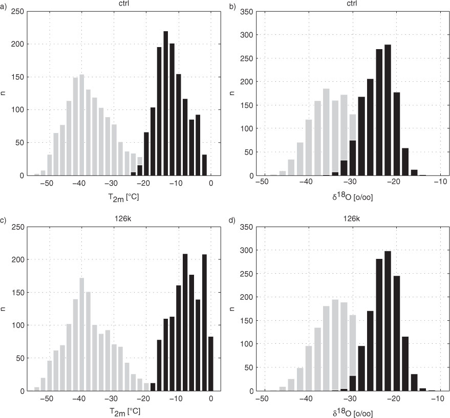
Fig. 4
(a) Histogram of monthly 2m temperature (T2m ) over Greenland above 1500 m for the control run (ctrl) during JJA (black) and DJF (grey). (b) Histogram of monthly δ 18O in precipitation over Greenland for the control run (ctrl) during JJA (black) and DJF (grey). (c) and (d) same as (a) and (b) but for the 126k time slice.
Table 3. Seasonal spatial slope (JJA and DJF means) and correlation (R 2) between δ 18O and temperature for land grid points north of 50°N (n=724) and for GIS above 1500 m (n=43)
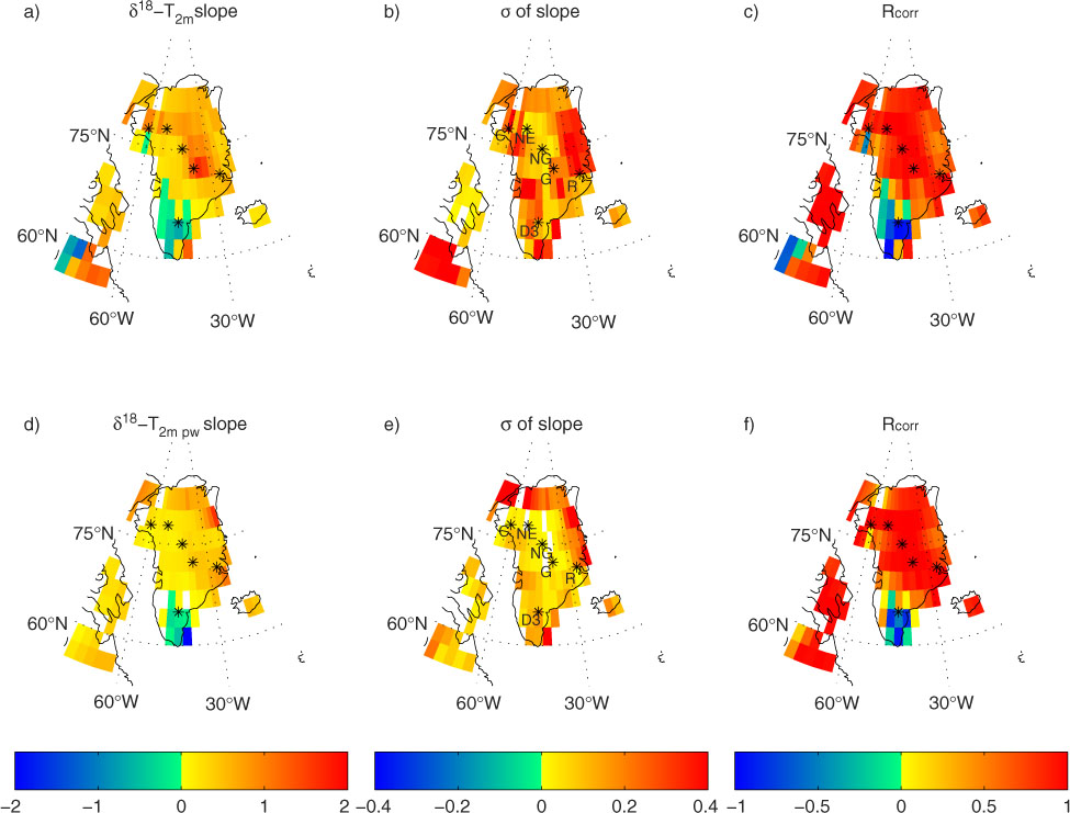
Fig. 5
(a) Slope between annual mean precipitation weighted δ 18O and annual mean temperature (T2m ) [‰/°C] calculated between the anomalies of the 115k, 122k and 126k time slices (b) one standard deviation on δ 18O–T2m slope (c) linear correlation of δ 18O and T2m between the time slices. (d) to (f) same as (a) to (c) but calculated using precipitation weighted annual mean T2m . The asterisk mark the ice core drill sites listed in Table 4 [Camp Century (C), NEEM (N), NorthGRIP (NG), GRIP (G), Renland (R) Dye-3 (D3)].
Table 4. δ 18O–temperature slope between Eemian time slices (115k, 122k, 126k) for ice core drill sites where Eemian ice has been recovered
[i] The slope is listed for JJA and DJF means, annual mean precipitation weighted δ 18O with annual mean 2m temperature (Annual) and annual mean precipitation weighted δ 18O with annual mean precipitation weighted 2m temperature (Pre. w. annual). R 2 listed in parenthesis. The ice core drill sites are marked in Fig. 5.
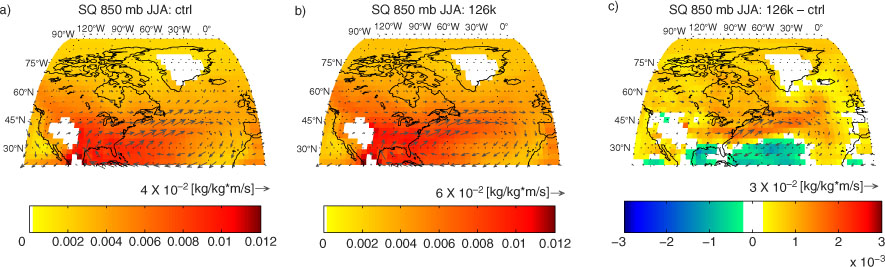
Fig. 6
(a) Specific humidity [kg/kg] of the 850 mb pressure level (shading) and vertically integrated vapour transport [kg/kg m/s] (arrows) for the control run (ctrl). (b) same as (a), but for the 126 kyr time slice (126k). (c) as in (b) but anomalies relative to the control run (126k-ctrl). Note the different scaling of the arrows showing the vapour advection. For vapour advection, only data for every second grid point are plotted.
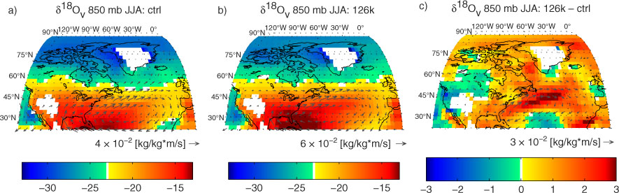
Fig. 7
(a) δ 18O of vapour [‰] for the 850 mb pressure level (shading) and vertically integrated vapour transport [kg/kg m/s] (arrows) for the control run (ctrl) (b) same as (a), but for the 126 kyr time slice (126k). (c) as in (b) but anomalies relative to the control run (126k-ctrl). The vapour advection plotted in this figure is the same as in Fig. 6.
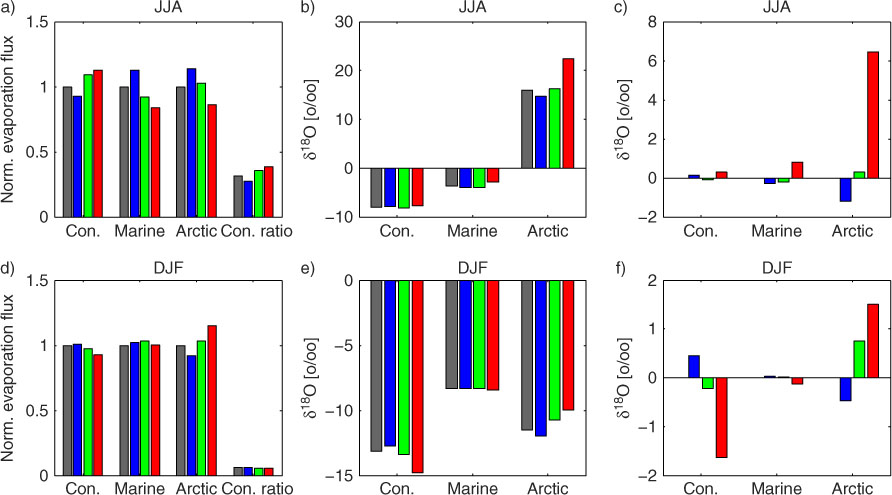
Fig. 8
(a) and (d) seasonal continental and oceanic evaporation fluxes relative to the control run, as well as the ratio of continental evaporation (Con. ratio) relative to total evaporation of the three regions. (b) and (e) seasonal δ 18O of evaporation fluxes [‰]. (c) and (f) seasonal anomalies in δ 18O of evaporation fluxes [‰]. The regions are defined as: North American (Con.) (land grid points 25°N <lat <70°N, 55°W <lon <170°W), North Atlantic (Marine) (ocean grid points 20°N <lat <60°N, 0°W <lon <95°W) and Arctic (Arctic) (ocean grid points lat >60°N) region. Bars represent fluxes for the different time slices: ctrl (grey), 115k (blue), 122k (green) and 126k (red).
Table 5. Ice core and modelled δ 18O for present (model: ctrl), the Eemian (model: 126k) and the Eemian anomaly (model: 126k-ctrl)
[i] See Johnsen and Vinther (2007) and Dahl-Jensen et al. (2013) for ice core data. The last column on the right lists the estimate of how much lower (ΔElev. [m]) the ice sheet was at each site during the Eemian. The calculation of ΔElev. is based on a modelled δ 18O lapse rate of −0.56‰/100 m for the 126k time slice and the difference between columns E ic -P ic and E mo -P mo .