
Fig. 1
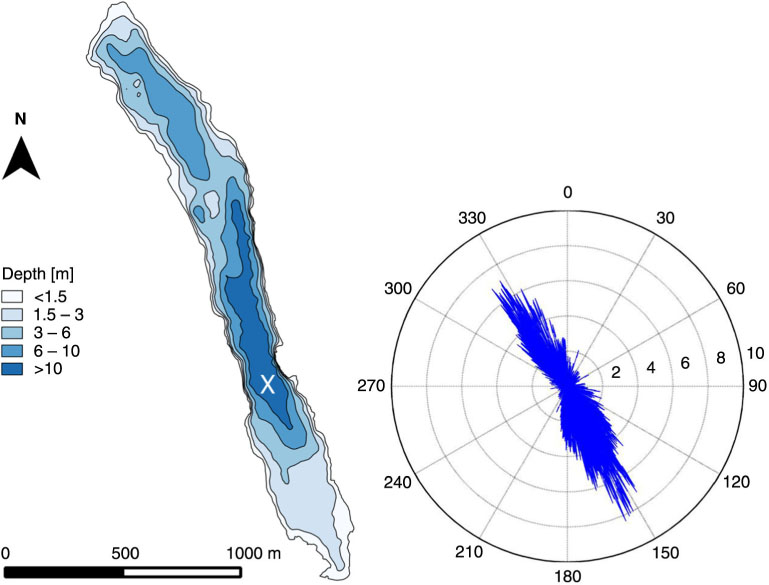
Contour map and wind rose for Lake Kuivajärvi. The location of the platform is indicated with the white cross. The wind directions in degrees are on the circumference and the lengths of the blue arrows indicate the wind speeds (m s−1).
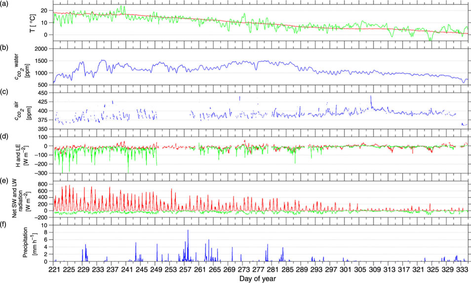
Fig. 2
(a) The measured surface water temperature (°C, red line) and air temperature (green), (b) the surface water CO2 concentration (ppm), (c) the atmospheric CO2 concentration (ppm), (d) the sensible (red) and latent (green) heat flux (W m−2), (e) the net shortwave (red) and longwave (green) radiation (W m−2), and (f) the precipitation (mm h−1). The x-axis is the day of year in all the graphs and the values are 0.5 hour averages.
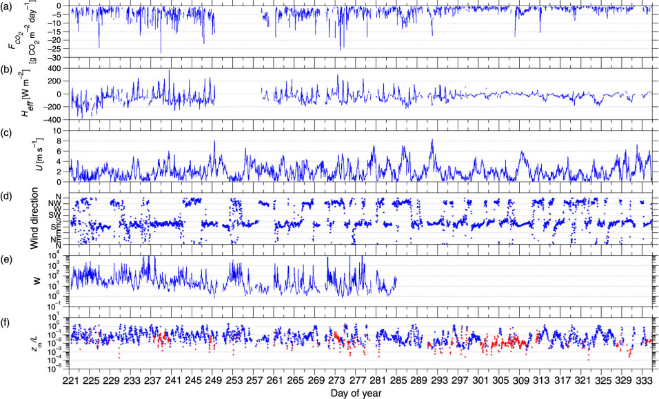
Fig. 3
Time series of half hour averages of (a) CO2 flux (g CO2 m−2 s−1), (b) the effective heat flux (W m−2), (c) wind speed (m s−1), (d) wind direction, (e) Wedderburn number, and (f) atmospheric stability parameter (positive values are on red and negative on blue).
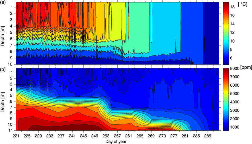
Fig. 4
(a) Isotherms (°C, 10-minute averages) and (b) isopleths of CO2 concentrations (ppm) in the water column during seasonal stratification. The CO2 data for 0–3 m are from Vaisala probes (0.5-hour averages) and for depths beyond that from headspace samples (weekly data). Temperatures were measured to a depth of 10 m, whereas the CO2 measurements were to 11 m.
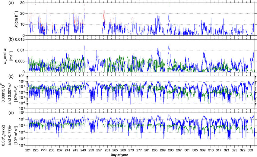
Fig. 5
Half hour averages of (a) k site (cm h−1, red dashed line) and k fp (solid blue line), (b) the aquatic friction velocity (blue line, m s−1) and the convective velocity (green, m s−1), and the wind parameter (blue) and the heat flux parameter (green) in k Uw (c, 106 m2 s−2) and k SR (d, 1012 m4 s−4).
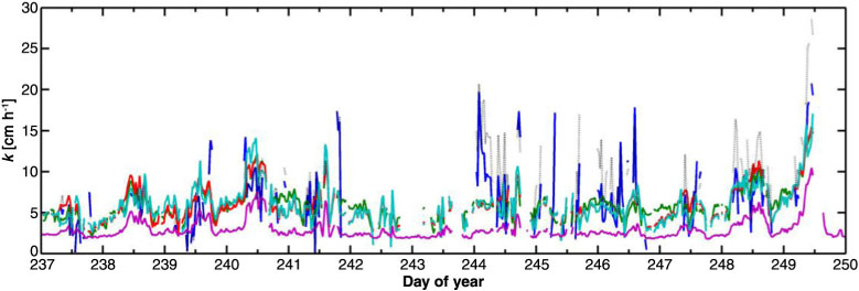
Fig. 6
Half hour averages of k site (black, dashed line, cm h−1) and k fp (blue line), and the modelled gas transfer velocities with k Uw (green), k SR (red), k RA (turquoise) and k CC (purple) during days 237–250.
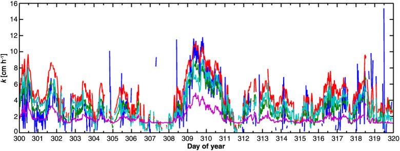
Fig. 7
Half hour averages of k fp (blue line, cm h−1), and the modeled gas transfer velocities with k Uw (green), k SR (red), k RA (turquoise) and k CC (purple) during days 300–320.
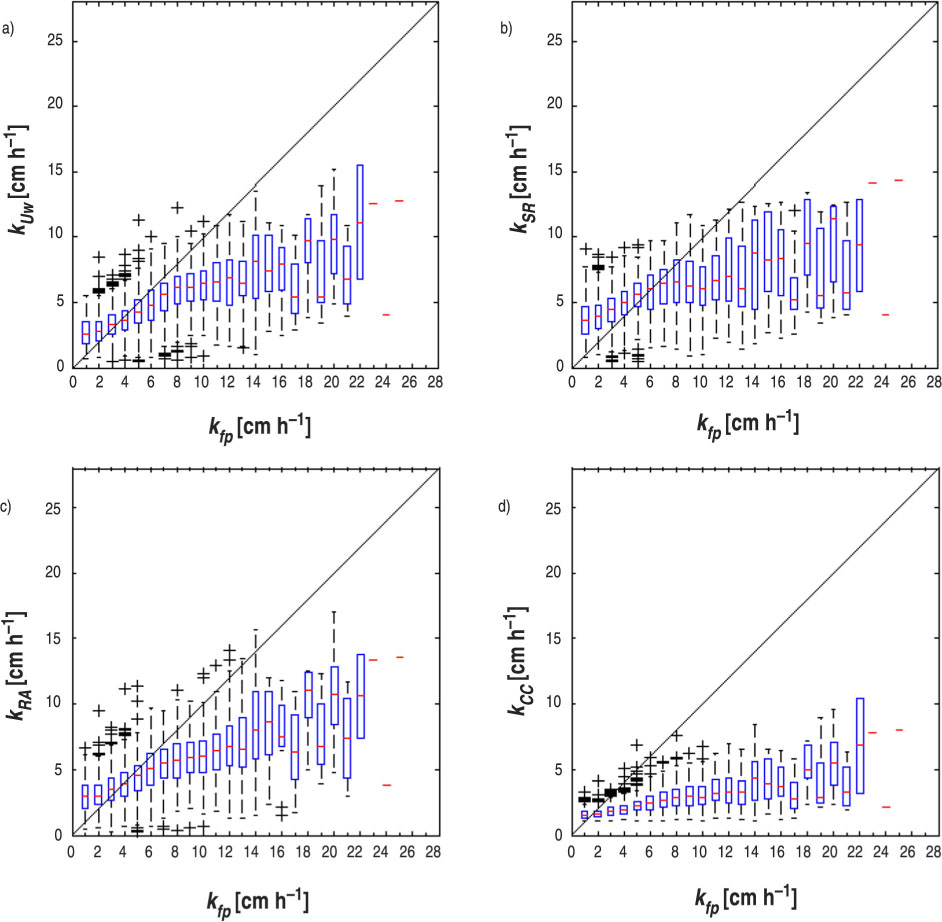
Fig. 8
The k fp (cm h−1), 0.5 hour averages, plotted against (a) k Uw , (b) k SR , (c) k RA and (d) k CC . The central red line of the box is the median, the edges of the box the 25th and 75th percentiles, the whiskers show the extreme values (±2.7σ) and the black crosses are remaining outliers. The data were binned by k fp , every 1 cm h−1, and the bins from 1 to 7 contain about 200 data points, bins 8–13 about 100, bins 14–18 about 50, and bins 19–25 less than 20 data points.
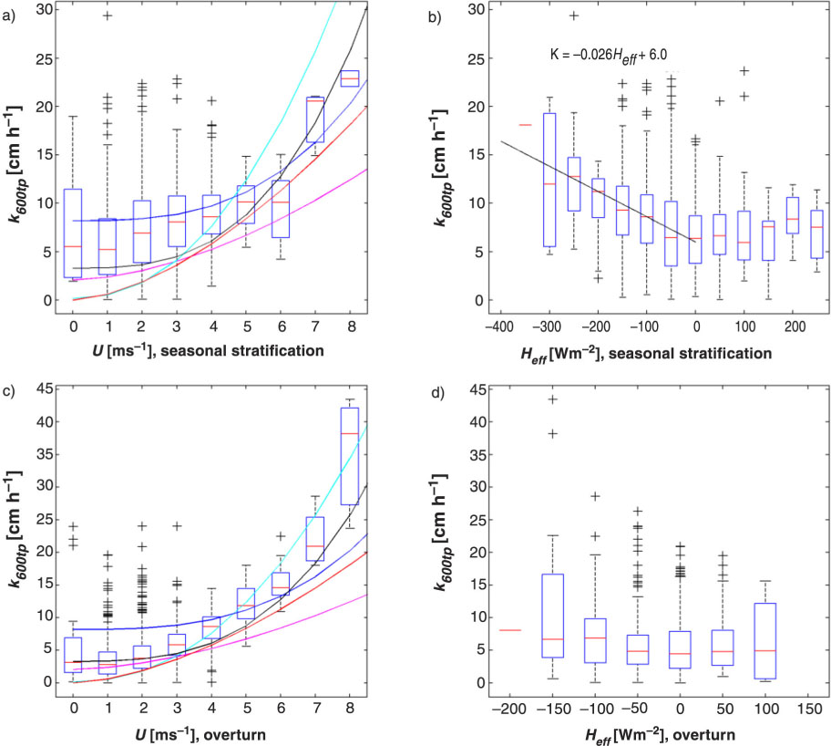
Fig. 9
The k 600fp (cm h−1), which is k fp after Schmidt number conversion, plotted against wind speed (m s−1) during (a) seasonal stratification (days 220–270) and (c) autumn overturn (days 290–335) and against the effective heat flux (W m−2) during (b) seasonal stratification and (d) autumn overturn. Also the regression of Cole and Caraco (1998) (purple line); Crusius and Wanninkhof (2003), k=0.168+0.228 (U 10 )2.2 (turquoise); Wanninkhof (1992), k=0.45(U 10 )1.64 (red); McGillis et al. (2001), k=3.3+0.026(U 10 )3 (black) and McGillis et al. (2004), k=8.2+0.014(U 10 )3 (blue) are presented in (a) and (c). The same statistical approach was used as in Fig. 8. In (a) and (c), the data were binned by wind speed, every 1 m s−1, and the bins from 0 to 8 contain about 300, 800, 600, 400, 200, 100, 30, 10 and 5 data points, respectively. In (b) and (d), the data were binned by heat flux, every 50 W m−2. The bins from −350 to 250 in (b) contain about 5, 10, 20, 50, 200, 400, 400, 200, 100, 50, 20, 10 and 10 data points, respectively, and the bins from −200 to 150 in (d) contain about 3, 50, 200, 500, 900, 100, 10 and 2 data points, respectively.
Table 1. The Pearson correlations between the measured k and the models (k Uw , k SR , k RA and k CC ), environmental forcing (wind speed, effective heat flux) and the parameters used in the models (aquatic friction velocity, convective velocity and buoyancy flux) during the whole measurement period, and separately during seasonal stratification and autumn overturn
[i] The correlations between k fp and H eff , w * and β are only shown when the lake was cooling. All of the correlations were significant at the 0.01 level (two-tailed) except with w * during autumn overturn. The N were 2150, 733 and 1029 for k Uw , k SR , k RA , k CC , U and u * , and 1591, 536 and 783 for H eff , w * and β during the whole period, seasonal stratification and autumn overturn, respectively.