Influence of water uptake on the aerosol particle light scattering coefficients of the Central European aerosol

3.1. Light scattering measurements at dry and elevated RH

The aerosol particle light scattering coefficient σ _sp was measured at three distinct wavelengths (λ=450, 550, 700 nm) using an integrating nephelometer (DryNeph; TSI Inc., Model 3563). This instrument performed measurements always at dry conditions (RH=11.2±2.7%, mean±standard deviation during the campaign) and is used as a reference to the humidified nephelometer. The spectral course of the particle light scattering coefficient can be described by the Ångström formula:

The humidified nephelometer (WetNeph) measured σ _sp at controlled and elevated RH between approx. 30 and 90% at the same wavelengths as the DryNeph. The WetNeph was connected to the same inlet as the DryNeph and was operated in parallel to it. It is technically described in detail in Fierz-Schmidhauser et al. (2010c) and only a brief description will be given here. The atmospheric aerosol is directed with a flow rate of 10 lpm into a humidifier, in which the aerosol is exposed to RH up to approx. 89%, followed by a dryer that dries the aerosol particles continuously down to approx. 50% RH. If the humidifier and dryer are turned off, the RH decreases further to approx. 30%. This combined set-up allows measuring both branches of the hysteresis curve. The residence time from the humidifier to the nephelometer cell is typically 1–3 seconds. σ _sp is then measured in an integrating nephelometer of the same brand and model as the DryNeph (TSI Inc., Model 3563), however modified for a better temperature and humidity control. The temperature and RH is measured at various points within the system using different sensors (Rotronic HygroClipS) and a dew point mirror (Edge Tech, Model 2000 Dewprime DF). The uncertainty in the nephelometer measurements of the scattering coefficient (approx. 10%; Anderson et al., 1996) and the uncertainty of the RH inside the nephelometer cell (1–2%; Fierz-Schmidhauser et al., 2010c) contribute to the measurement uncertainty of f(RH). Both error sources combined give a relative uncertainty of Δf(RH=85%)≈20% for a very hygroscopic aerosol, which will decrease for less hygroscopic aerosol or smaller RH (and vice versa).

The WetNeph was set to measure in a constant RH mode for the first period of the campaign and set to measure in the humidogram mode for the second part of the campaign. A full humidogram (hydration and dehydration) took approximately 2 hours. The constant RH mode allows to better investigate the temporal evolution of f(RH), like diurnal cycles, while the humidogram mode characterises the shape of the f(RH) curve and reveals information on possible hysteresis behaviour.

The temperature of the two nephelometer systems was kept low (below approx. 23°C) to avoid losses due to the evaporation of ammonium nitrate (Bergin et al., 1997). The integration time of both nephelometers was set to 1 minute.

3.2. Hygroscopicity tandem differential mobility analyser

Hygroscopic particle growth factors were measured by a custom-built hygroscopicity tandem differential mobility analyser (H-TDMA). This instrument had been deployed for several years to characterise ambient aerosols (Massling et al., 2003), but was upgraded for continuous measurements at Melpitz during 2008 and 2009 according to the specifications outlined by Massling et al. (2011). During field operation, the H-TDMA was regularly checked for a correct particle sizing in the two differential mobility analysers. The H-TDMA performance was also verified by intermittent measurements of the hygroscopic growth factor of pure ammonium sulphate particles.

The H-TDMA allows the determination of the hygroscopic growth factor g(RH), which is defined as the diameter D _{p, wet} at a certain elevated RH divided by its dry diameter D _{p, dry} :

Equation 3 can be parameterised using a one-parameter relationship which has been proposed, e.g. by Petters and Kreidenweis (2007):

The hygroscopic growth factor can also be calculated using the chemical composition measurements of multi-angle absorption photometer (MAAP) and aerosol mass spectrometer (AMS) (see Sections 3.3 and 3.5) of the different aerosol components and applying the Zdanovskii–Stokes–Robinson (ZSR) mixing rule (Stokes and Robinson, 1966). Black carbon (BC) is assumed to be insoluble (g=1), while the value of g for the organic fraction was taken from Sjogren et al. (2008) who characterised the hygroscopic growth of aged organic aerosol (e.g. g=1.19 for D _p,dry =100 nm and RH=85%). The values of the retrieved salts and acids are taken from Topping et al. (2005). We refer to Fierz-Schmidhauser et al. (2010a); Gysel et al. (2007) for more details on the calculation and uncertainty.

3.3. Light absorption measurements

The aerosol particle light absorption was determined using a MAAP (Thermo Scientific Inc., Model 5012), which measures the light attenuation and backscattering of aerosols (at λ=637 nm, Müller et al., 2011) which are deposited on a filter. An internal radiative transfer code is applied to calculate the fraction of light absorbed by the deposited particles (Petzold and Schönlinner, 2004). The aerosol absorption coefficient σ _ap is retrieved by multiplying the reported BC concentration with the internal set value of the mass absorption cross-section of 6.6 m²g⁻¹.

3.4. Number size distribution measurements

Particle number size distributions were measured by a dual mobility particle size spectrometer (custom-built by TROPOS and traditionally called TDMPS). The Melpitz TDMPS (Birmili et al., 1999) consists of two mobility analysers covering a total particle size range of 3–800 nm (electrical mobility diameter), but was updated to circular sheath flow regulation according to the EUSAAR/ACTRIS recommendations (Wiedensohler et al., 2012). Multiple charge correction was performed according to Pfeifer et al. (2014).

The larger diameter size ranges were characterised using an optical particle size spectrometer (OPSS; Dust Monitor 1.108, Grimm GmbH). The OPSS determines the particle number size distribution (optical equivalent diameter) in 15 different channels between D _p >0.3 µm and D _p >20 µm. It classifies the particles concerning their light scattering properties and uses light that is emitted from a laser diode at λ=780 nm. The OPSS is calibrated using polystyrene latex particles (PSLs). Since the refractive index of the atmospheric aerosol particles can differ from the PSL value, the particle number size distribution of the OPSS was corrected for different complex refractive index values (see e.g. Bukowiecki et al., 2011).

The measured particle number size distribution branches of TDMPS and OPSS were merged at D _p =800 nm as the joint particle diameter channel. The first four OPSS channels were excluded with D _p =900 nm being the first OPSS measured channel. The OPSS and TDMPS particle number size distributions agree well within the overlap region (N _OPSS(350–725 nm)=0.93*N _TDMPS(365–800 nm)+4.92), R ²=0.97; R ²: squared Pearson's correlation coefficient).

3.5. Chemical composition measurements

The chemical composition of the particles was characterised using an Aerodyne high resolution time-of-flight AMS (Aerodyne Research, U.S.A.). The instrument is described in detail e.g. in DeCarlo et al. (2006); Canagaratna et al. (2007). The AMS measures the chemical composition of non-refractory particles with diameters smaller than 1 µm (vacuum aerodynamic particle diameter). A collection efficiency of 0.5 was determined for the AMS using estimated mass concentrations from the TDMPS and the chemical analysis of filter samples Poulain et al. (2011).

A collection efficiency of 0.5 was determined for this AMS using the particle number size distribution and the chemical analysis of filter samples. Because soot, crustal material and sea-salts cannot be detected, the AMS is commonly considered to provide non-refractory PM₁ aerosol particle chemical composition (Canagaratna et al., 2007). By combining the MAAP-based BC measurements and the AMS chemical composition, a highly time resolved and comprehensive picture of the submicron chemical particle composition can be provided. During 2008 and 2009, the same AMS was installed for different campaigns at Melpitz and the results are presented in Poulain et al. (2011), who also discuss the results of the AMS measurements performed during our time period in further detail.

In parallel to the AMS and MAAP measurements, aerosol particles were also collected by daily PM₁₀ High Volume DIGITEL filer samples (Digitel Elektronik AG, Hegnau, Switzerland) from midnight to midnight. Filters were weighed to obtain concentrations of the total particle mass and water soluble inorganic cations and anions as well as OC/EC. Details on the different analytical methods and results for can be found in Spindler et al. (2010).

5.1. WetNeph analysis

The campaign at Melpitz was carried out from 23 February until 30 March 2009. The WetNeph was set to measure in the constant RH mode for the first half of the campaign (24 February–11 March), while it measured humidograms (periodically changing RH) in the second half of the campaign (11–26 March). Example humidograms of f(RH) at λ=550 nm are shown in Fig. 1a–d together with 72-hour air mass back trajectories (FLEXTRA, Stohl et al., 1995; Stohl and Seibert, 1998) for the specific time periods. Shown are the hydration and dehydration scans of f(RH) (1 minute values, green points) together with a parameterisation of the upper and lower branch (see below). The particle surface size distribution measured by the TDMPS and by the OPSS as well as the mean submicron mass ratios measured by the AMS and MAAP are shown for the same time periods in Fig. 1f–i. Figure 1a shows an example of westerly air masses with a smooth increase of f(RH) with increasing RH. The corresponding surface size distribution, which is generally relevant for the scattering properties, shows that the main contribution comes from particles in the fine mode at D _p ≈300 nm, while the fine mode chemical composition is dominated by organics and NO₃ (Fig. 1g). The second example (Fig. 1b) shows almost no increase of f(RH) with increasing RH (hydration of the aerosol) until approx. 55% RH where f(RH) suddenly increases to about 1.5 and further rises with increasing RH. This deliquescence behaviour (sudden transition from the solid to the liquid state of the majority of the particle population) is attributed to transported sea salt, as can be seen in the back trajectories which indicate a transport of air from the North Sea towards Melpitz. In the dehydration mode (decreasing RH; max RH set in humidifier and drying the aerosol back to lower RH~50%), the deliquescence RH is passed and particles will become (partially) solid at a lower RH. This RH point (efflorescence) cannot be directly measured due to the limitations of the drying system, which only dries until approx. 50% RH. It should be mentioned that the observed deliquescence RH measured by the WetNeph is not identical with the thermodynamical deliquescence RH, since the particles are exposed to the highest RH in the humidifier and the RH decreases until the particle light scattering properties are measured inside the nephelometer (see Fierz-Schmidhauser et al., 2010c). The surface size distribution for the same period (Fig. 1h) clearly shows an increased coarse mode. As mentioned above, the AMS can only detect non-refractory material and thus cannot directly determine the sea salt contribution, although the chloride fraction in Fig. 1h is slightly enlarged compared to the other examples. Figure 1c shows a humidogram characterised by low values of f(RH), probably due to an increased influence of anthropogenic aerosol particles. This can be seen in the corresponding submicron mass ratio (Fig. 1i), where the BC and organic mass fraction make up approx. 60% of the total submicron mass. Additionally, the particle surface size distribution shows an increased contribution of Aitken mode particles (D _p ≈10–100 nm), which is typical for fresh anthropogenic pollution. The humidogram in Fig. 1d shows a similar behaviour as Fig. 1a, but with an increased curvature and higher f(RH) values. The chemical composition reveals an increased nitrate fraction and less contribution from organics and BC, which are compared to NO₃ also less hygroscopic. The dominance of rather sharp mode at D _p ≈300 nm characterises the particle surface size distribution as depicted in Fig. 1j.

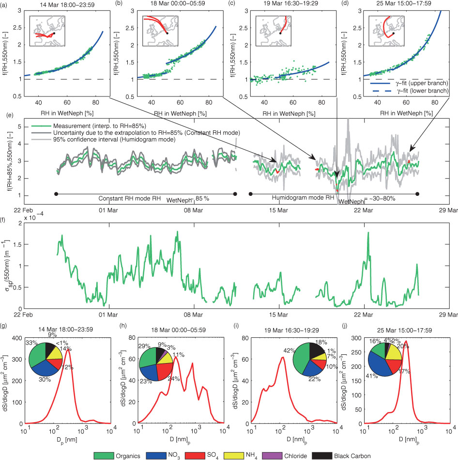
Fig. 1

The humidograms were parameterised using an empirical equation that has been used in previous studies (e.g. Clarke et al., 2002; Carrico et al., 2003; Zieger et al., 2011) to describe the RH dependency of f(RH):

The time series of f(RH) at 85% RH and λ=550nm is depicted in Fig. 1e together with the dry particle scattering coefficient in Fig. 1f. The humidograms were extrapolated to RH~85% using eq. 5. During the constant RH mode, the RH inside the WetNeph was measured at 82.7±1.0% (mean±standard deviation), with an average f(RH) of 2.69±0.29. The measured f(RH) values were extrapolated to RH=85% by taking a constant value for a in eq. 5 (a=0.9±0.1 at λ=550 nm; mean and standard deviation of entire campaign). The resulting uncertainty from this extrapolation is seen in Fig. 1e as grey lines and is calculated by taking the upper and lower bonds of a (eq. 5). The uncertainty for the humidogram period is calculated by taking the upper and lower 95% confidence bonds for the fit parameters a and γ for the extrapolation to RH=85%. Large uncertainties during the humidogram mode are mainly due to low concentrations and/or changing air masses during the 2-hour averaging time, which resulted in a higher fit-uncertainty (e.g. 20 March). The time series in Fig. 1e shows a high variability of f(RH) (see Table 1 with mean and percentile values of f(RH=85%) for the entire campaign). A slight spectral dependency of f(RH) can be observed for the higher values (see 90th percentile values in Table 1); however, this difference is clearly below approx. 10% (at RH=85%) and therefore the focus in the following discussion will be kept on the 550 nm wavelength. However, it should be mentioned that the wavelength dependency of f(RH) was reproduced and verified with Mie calculations using the measured size distribution and PM₁ chemical composition (see Section 5.3).

The hysteresis behaviour in f(RH) is observed, when non-anthropogenic influenced sea salt with large fractions of sodium chloride was present. To illustrate the frequency of observed hysteresis, the difference of f(RH=55%, 550 nm) of the upper branch minus the f(RH=55%, 550 nm) of the lower branch is shown in Fig. 2 together with the sodium chloride (NaCl) mass fraction of the PM₁₀ daily filter samples. An increased difference of the two f(RH) branches at RH=55% corresponds to an increased NaCl mass concentration, which can be interpreted as a tracer for transported sea salt at Melpitz (Spindler et al., 2010). One particular sea salt transport event from the Northern Sea was observed on 18 March 2009, which resulted in a clear hysteresis in the measured humidogram (see also humidogram and trajectories in Fig. 1b).

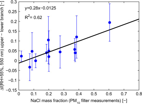
Fig. 2

Figure 3a shows 72-hour air mass back trajectories colour-coded with the f(RH=85%, 550 nm) measured at the time the air parcel arrived at the site, while Fig. 3b and 3c show the same trajectories but now colour-coded by the inorganic mass fraction determined by the AMS and MAAP measurements (see Section 5.2) and colour-coded by the mean surface area particle diameter measured by the TDMPS and OPSS. Westerly air masses dominated during the campaign. Increased values of f(RH=85%, 550 nm) were connected to an increased inorganic particle mass fraction. Very low f(RH=85%, 550 nm) values at approx. 1.1–1.2 were simultaneously measured with low inorganic particle mass fractions and small mean surface area particle diameters, typically when the air arrived from north-east to Melpitz with a transport of accumulated anthropogenic air masses. In contrast to other sites (e.g. Jungfraujoch or Mace Head, see Fierz-Schmidhauser et al., 2010b; Zieger et al., 2012), no distinct dependency on large scale air mass transport phenomena or air mass sectors was observed at Melpitz and rather a high variability in f(RH=85%, 550 nm) was characteristic for this site.

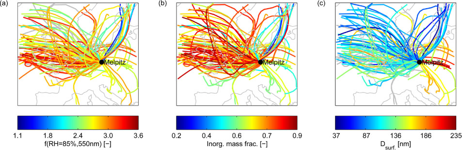
Fig. 3

5.2. Chemical composition determining f(RH) at Melpitz

The colour-coded trajectories (Fig. 3) already point towards the fact that the scattering enhancement is mainly correlated with the inorganic mass fraction and is less dependent on the mean surface area particle diameter. The main chemical particle mass fractions versus f(RH=85%, 550 nm) are shown in Fig. 4. They are calculated by dividing the individual particle mass concentrations of organic, nitrate, sulphate, ammonium (all measured by the AMS) and BC (measured by the MAAP) by the sum of all. The inorganic particle mass fraction is calculated by dividing the sum of nitrate, ammonia and sulphate concentration by the sum of all (incl. BC). Organics and BC mass fractions are clearly anti-correlated with f(RH=85%, 550 nm) due to the lower hygroscopicity of these compounds, while inorganic substances clearly show a positive correlation with f(RH=85%, 550 nm) due to their hygroscopic characteristics. The ammonium mass fraction shows a similar strong (positive) correlation (R ²=0.64) as the total inorganic mass fraction (R ²=0.57), while the individual nitrate and sulphate mass fractions are only weakly correlated with f(RH=85%, 550 nm). This is mainly attributed to the fact that ammonium is the common ion of the two major salts (ammonium sulphate and ammonium nitrate) and can be regarded as a proxy for the total inorganic content. Ammonium sulphate and ammonium nitrate also have different hygroscopic properties. The sum of the sulphate and nitrate mass fractions shows as expected a clear positive correlation with f(RH=85%, 550 nm) (slope 2.9, R ²=0.53). Figure 4 clearly demonstrates that a (mean) particle chemical composition (e.g. the inorganic fraction) needs to be known to predict f(RH) at Melpitz. The orthogonal linear regressions were calculated according to York et al. (2004) by taking the error of the measurements into account, which allows retrieving an uncertainty of the slope and intercept given in Fig. 4. For the AMS and BC measurements, the standard deviation of the 1-hour averages was taken, while the uncertainty of f(RH=85%, 550 nm) was calculated as described above. The f(RH) at a different RH can now be estimated from the chemical mass fractions using the equations in Fig. 4 together with eq. 5 and a fixed intercept of a=0.9. However, one has to be aware that eq. 5 is a purely empirical equation with clear limitations for very low (RH<30%) or high (RH>90%) values of RH, because the upper and lower RH ranges were not covered by the measurements (30<RH<90%). In addition, possible hysteresis effects (see Fig. 1b) are not captured using a fixed intercept and γ-value to calculate f(RH).

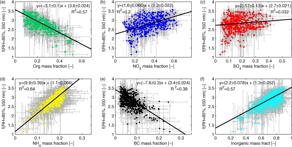
Fig. 4

Figure 5 shows the squared correlation coefficient and the sign of the correlation of f(RH=85%, 550 nm) with different in-situ aerosol particle parameters. As already seen above, the f(RH=85%, 550 nm) is clearly correlated with the inorganic mass fraction and anti-correlated with the organic mass fraction or the BC mass fraction. There is no significant correlation with any size parameters, such as the surface area concentration of the coarse mode fraction S_CM/S_tot (measured by the OPSS and TDMPS), the total particle surface area fraction S_tot or the Ångström exponent of the particle light scattering coefficient at dry conditions (see eq. 2). This implies that the aerosol particle chemical composition (or at least a proxy of it) needs to be known to predict f(RH) from other continuous monitoring measurements. The rather weak correlation of the hygroscopic growth factor g with f(RH) (R ²=0.2) is most probably due to the short operation period of the H-TDMA and the fact the H-TDMA only measures at the dry diameters below 265 nm and therefore will not always cover all optically relevant size ranges such as a hygroscopic coarse mode, e.g. due to transported sea salt or non-hygroscopic mineral dust (Zieger et al., 2011).

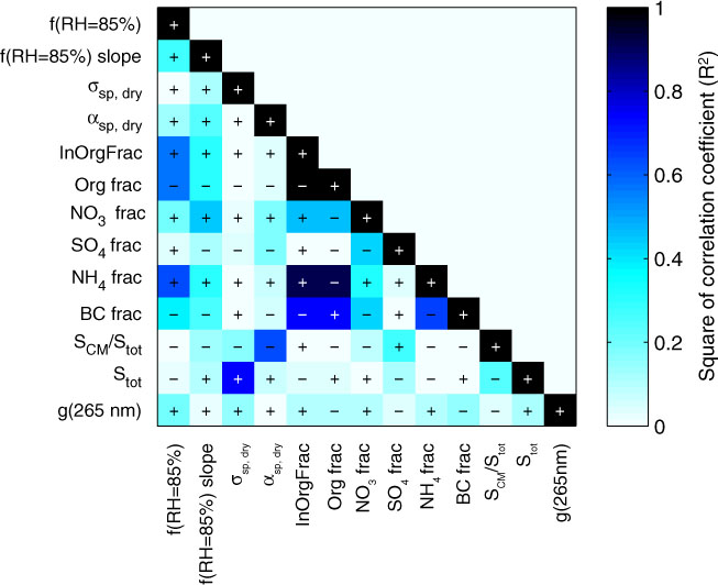
Fig. 5

5.3. Optical closure study

The different in-situ measurements were checked for consistency with respect to f(RH) and σ _sp by performing Mie calculations (see Section 4). As mentioned above, the correct OPSS sizing depends on the refractive index of the particles. The OPSS was calibrated by the manufacturer with PSL particles. However, the refractive index of PSL (m _PSL=1.586) differs from the ambient aerosol values. In particular, the imaginary part of m is usually not negligible. The particle number size distributions of the OPSS were therefore corrected by assuming the real part of the dry refractive index to be 1.5 (close to the value of ammonium sulphate and best found to fit with the number size distribution measurements of the TDMPS) and by changing the imaginary part between 0 and 0.02i. This range is also supported by a recent analysis of long-term impactor measurements (Spindler et al., 2012). The refractive index m_AMS was retrieved from AMS and MAAP measurements (see Section 4) with (m _AMS(550 nm)=(1.54±0.0076)+(0.031±0.016)i (mean±standard deviation for entire campaign). The real part is close to the value of ammonium sulphate, while the imaginary part is close to the range estimated from the impactor measurements for the different size ranges (0.019–0.044i).

The Mie calculations were repeated for the particle light scattering coefficient at dry conditions and the comparison with the measured value (at λ=550 nm) of the DryNeph is depicted in Fig. 6a. The centre points are the results for the OPSS correction with m _OPSS=1.5+0.01i, while the error bars give the range of the calculated σ _sp for the other refractive indices and the non-corrected OPSS. The error bars in the x-direction give the standard deviation of the 1-hour mean values. The bivariate linear regression and the R ² show a very good agreement with the DryNeph measurements and only a slight influence of the OPSS size distribution, showing the minor influence of the coarse particle fraction to the particle light scattering coefficient at the wavelengths used in this study and at this site. Figure 6b (lower row) shows the comparison as a box plot of the percentile difference between measured and predicted value (100%×(predicted-measured)/measured). The central red mark in Fig. 6d is the median, the edges of the box are the 25th and 75th percentiles, the error bars show the extent to the most extreme data points that are not considered as outliers, while the outliers are plotted individually (red crosses). In addition, the number of points of the compared 1-hour averages is given. Fig. 6b reveals that the interquartile range of ${\sigma }_{\text{sp}}^{\text{dry}}$ can be calculated with a deviation of <10% using the refractive index retrieved from the AMS and MAAP.

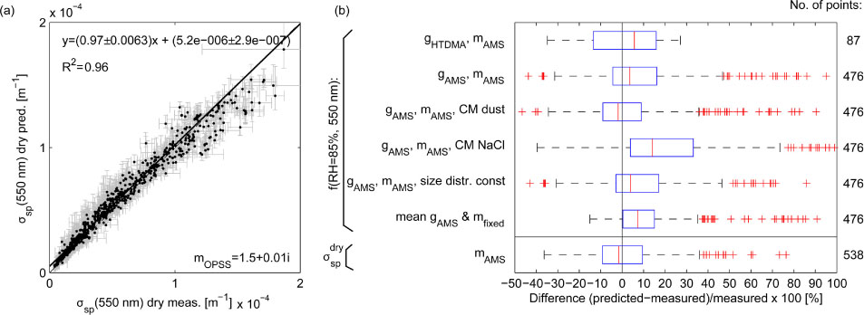
Fig. 6

f(RH=85%, 550 nm) in Fig. 6b is also predicted using the hygroscopic growth factor and the refractive index derived from the AMS and MAAP measurements (see Sections 3.2 and 4). In addition, the f(RH=85%, 550 nm) is calculated using the hygroscopic growth factor of the H-TDMA (with less data points of the H-TDMA being available for our period) and the refractive index from the AMS and MAAP. g for ${\text{D}}_p>{\text{D}}_{p,\text{d}ry}^{\text{max}}$ was assumed to be equivalent with g measured at the largest dry diameter ${\text{D}}_{p,\text{d}ry}^{\text{max}}$ of the H-TDMA. Both predictions are compared to the measured values of the WetNeph. The result is seen in the first two rows of Fig. 6b (row 1: g from H-TDMA, row 2: g from AMS and MAAP). The calculated values were successfully predicted and lie within the same range as the measured ones; however, the comparison shows a moderate variability and small squared correlation coefficients R²~0.1–0.12 (not shown). This can generally be explained by propagating uncertainties of the input parameters (e.g. the uncertainties in the combined size distribution) and in the assumptions of the Mie calculations (spherical particles, internal and homogeneous mixture). The interquartile range of f(RH) using g from the AMS or H-TDMA can be predicted with a deviation of <15%, while the median of the percentile difference lies between 3 and 5%. The comparison to the H-TDMA measurements was influenced by the low number of measurement points during the observation period due to instrumental reasons, which probably explains the low R ² value compared to similar calculations at other sites (e.g. Zieger et al., 2011).

To further investigate the sensitivity of the different input parameters, the Mie calculations were repeated with different assumptions (3rd to 6th row in Fig. 6b):

1. The coarse mode (CM; with D _p >1 µm) was assumed to consist of mineral dust particles (g=1 and m from Hess et al. (1998); Fig. 6b, row 3).

2. The CM was assumed to consist of pure sodium chloride particles (g and m were taken from the Seinfeld and Pandis (2006) and Topping et al. (2005); Fig. 6b, row 4).

3. The particle number size distribution was kept constant (mean value of TDMPS and OPSS of entire campaign; Fig. 6b, row 5).

4. A fixed value of m=1.5+0.005i and g(RH=85%)=1.53 was assumed (mean value derived from AMS and MAAP measurements; Fig. 6b, row 6).

The closure results for the four example humidograms are shown separately in Fig. 7. It can be seen that the curvatures of f(RH) are well captured in almost all cases; however, substantial offsets and distinct artefacts occur for the different model assumption. This generally illustrates the limitations of the closure approach:

1. The importance of the coarse mode. The coarse mode clearly influenced f(RH) at Melpitz, as can be seen in the sea salt influenced humidogram (Fig. 7b). The chemical composition was only adequately determined by the AMS (and MAAP) for the fine mode, while assumptions had to be made for the coarse mode. Figure 7b therefore shows an overprediction for the NaCl and a clear underprediction for the mineral dust composed coarse mode (dashed blue and yellow curves). If the properties of the fine mode are extrapolated to the coarse mode, the result will also be an underprediction of f(RH). In addition, the particle number size distribution of the coarse mode was measured by an OPSS, which is limited in its resolution and correct sizing (see above). This is seen in Fig. 1h, where the particle surface size distribution is depicted for the same period. In fact, the clear anthropogenic influenced humidogram (Fig. 7c) also reveals a small increased coarse mode (see Fig. 1i), which explains the modelled differences between the NaCl and dust coarse mode cases (dashed blue and yellow curves in Fig. 7c).

2. The assumption on an internally and homogeneously mixed aerosol. This is crucial assumption, which is probably not fully appropriate for the aerosol encountered at Melpitz. The aerosol chemical composition, and with this the aerosol hygroscopicity and complex refractive index as model input parameters, will vary with particle size. In addition, only the upper branch of the fully deliquescent aerosol can be modelled, which can lead to a clear overestimation of f(RH) at low relative humidities (RH <50%), when the aerosol is partially in the solid or liquid phase. This is clearly seen in Fig. 7b for the sea salt case, but may also be the reason for the slight overestimation of the predicted f(RH) for the other cases in Fig. 7 for RH <50% for an externally mixed aerosol.

3. Spherical particles. Further limitations may result from the assumption of spherical particles, which has to be taken when optical particles are calculated by Mie theory. Sea salt and mineral dust, however, are not spherical and therefore Mie theory cannot be used (Nousiainen, 2009). Nevertheless, for measurements with an integrating nephelometer, the error in σ _sp is assumed to be <5% for particles with D _p<1 µm, but up to 30% for cubic particles >1 µm (Chamaillard et al., 2003).

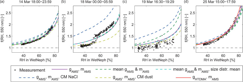
Fig. 7

We can conclude that the Mie calculations clearly show that the in-situ measurements are generally consistent, despite the large variation of the predicted f(RH), which can be explained by the uncertainty and limitations of the input data (e.g. PM₁ size cut of AMS) and the assumptions being made (spherical particles, internal and homogeneous mixture, etc.).

5.4. Context to previous studies

Continental and polluted air masses were also observed with the same WetNeph instrument at Cabauw, The Netherlands (Zieger et al., 2010) and at Mace Head, Ireland (Fierz-Schmidhauser et al., 2010b). Compared to these two sites, Melpitz had the unique opportunity to add highly time resolved aerosol chemical analysis of the AMS to the analysis of f(RH). At Cabauw, continental air masses coming from the east or the south had on average a value of f(RH=85%, 550 nm)=1.86±0.17 and 2.25±0.16, respectively (mean±standard deviation). In Mace Head, the air masses coming from the polluted (anthropogenic influenced) wind sector showed on average a value of f(RH=85%, 550 nm)=1.8±0.26. The f(RH=85%, 550 nm)-ranges for maritime aerosol varied largely at Cabauw and Mace Head, ranging from 1.95±0.14 for heavily polluted maritime aerosol to 3.38±0.31 for pure maritime aerosol. The Melpitz retrieved value (f(RH=85%, 550 nm) ≈2.5) for the few maritime influenced periods would be included in this range. The comparison of f(RH) values of other studies is difficult to achieve due to very different instrumental set-ups, especially with respect to the applied particle size cuts (PM₁, PM₁₀ or no size cut), different RH ranges or different wavelengths. While there are more studies that present f(RH) for marine, dust or strong anthropogenic influenced aerosol (see references above), only few suitable studies exist for continental aerosol types. However, Koloutsou-Vakakis et al. (2001) present f(RH) values from a continental site in the US (Bondville) with the same nephelometer type and also state a parameterisation to retrieve f(RH) at different RH which results in 1.58 for RH=85% and λ=550 nm. This value is substantially lower than the measured average value here of 2.77±0.37 for continental aerosol which could be explained by smaller particles or more hygroscopic particles (or a combination of both) encountered at Melpitz. The corresponding high inorganic mass fraction of the submicron refractory aerosol of 0.71±0.13 supports this hypothesis. A minor but not negligible effect is the RH of the reference nephelometer. At Melpitz, the RH inside nephelometer was very low, with RH=11.2±2.7% (mean±standard deviation during the entire campaign), while other studies often used RH<40% as a reference since organic dominated aerosol particles already take up water at low RH. For example, Sjogren et al. (2007) retrieved a value of g(40%)=1.05 at the Jungfraujoch (Switzerland) which can cause an overestimation of the apparent dry scattering coefficient by approx. 10% which will propagate to the retrieved f(RH). Particle losses in the humidifier and systematic nephelometer offsets can be an additional source for a systematic underestimation of f(RH). The achieved closure supports the values found here of f(RH), since they were reproduced from highly time resolved chemical and particle size distribution measurements. In general, particle size and chemical composition are both important for f(RH). In the Arctic for example, compensating effects of size and hygroscopicity were observed, e.g. small but less hygroscopic particles eventually had the same magnitude in f(RH) as large but more hygroscopic particles (like sea salt) with an average value of f(RH=85%, 550 nm)=3.24±0.63 (Zieger et al., 2010).