
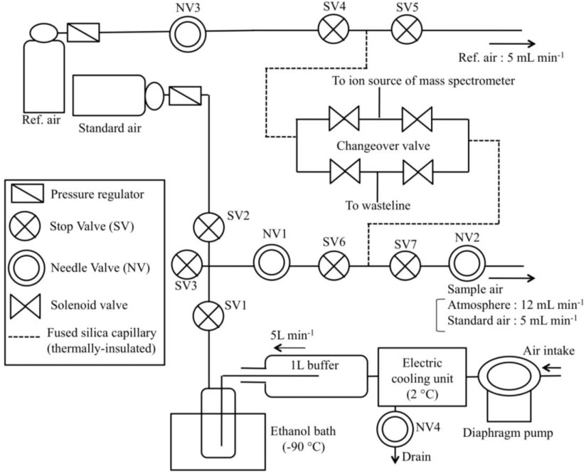
Fig. 1
Schematic diagram of the continuous measurement system for the atmospheric δ(O2/N2), δ(Ar/N2) and δ(CO2/N2).
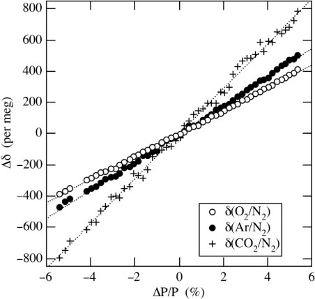
Fig. 2
Dependence of the measured δ(O2/N2), δ(Ar/N2) and δ(CO2/N2) on the relative pressure change (ΔP/P) between the sample air and the reference air to the pressure of the reference air at their introduction into the mass spectrometer.
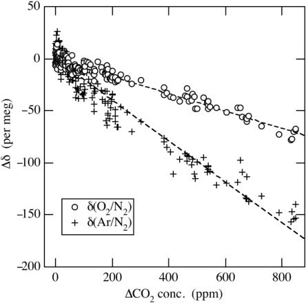
Fig. 3
Changes of the measured δ(O2/N2) and δ(Ar/N2) values of the air sample dependent on its CO2 concentration. ΔCO2 represents the difference between the CO2 concentration of the air-based CO2 standard air after and before adding pure CO2 (see text).
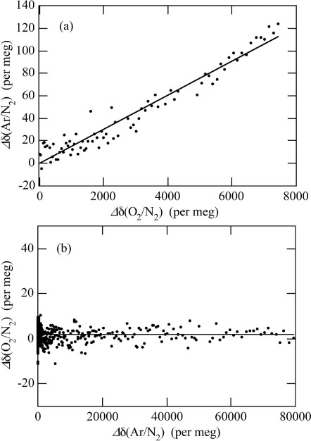
Fig. 4
(a) Change of the measured δ(Ar/N2) of the sample air dependent on its δ(O2/N2). (b) Same as (a) but for change of the measured δ(O2/N2) of the sample air dependent on its δ(Ar/N2). Δδ(Ar/N2) [Δδ(O2/N2)] is the difference between the measured δ(Ar/N2) [δ(O2/N2)] of the air-based CO2 standard air after and before adding pure O2 or Ar (see text).
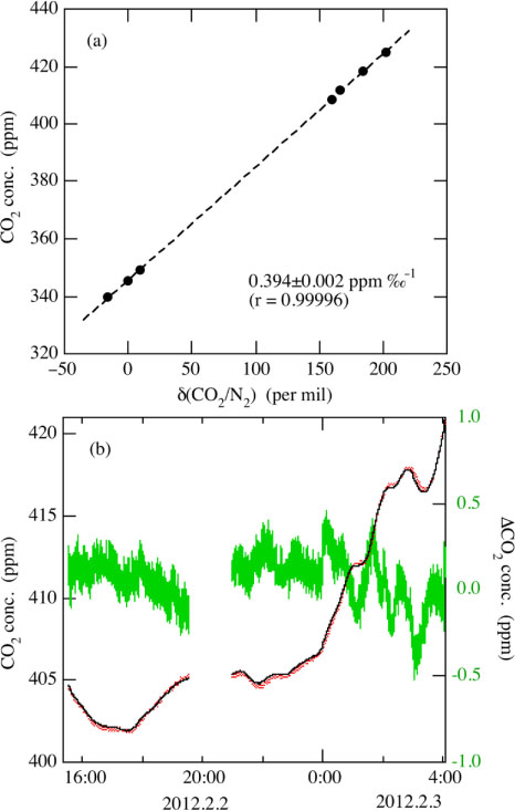
Fig. 5
(a) Relationship between δ(CO2/N2) of standard air measured using the mass spectrometer and CO2 concentration measured using a non-dispersive infrared analyser (NDIR). δ(CO2/N2) data were obtained on different days during May 17–June 11, 2012. (b) Atmospheric CO2 concentrations observed at Tsukuba, Japan using the mass spectrometer (black solid line) and a NDIR (red dots), and their differences (green line).
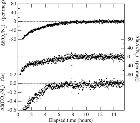
Fig. 6
Typical analytical results of the δ(O2/N2), δ(Ar/N2) and δ(CO2/N2) of a standard air against a reference air. Data are shown as deviations from the average values for the period after 8 hours analyses.
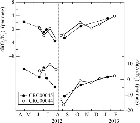
Fig. 7
Temporal changes of the δ(O2/N2) and δ(Ar/N2) of the standard air (CRC00045 and CRC00044) against a reference air. Data are shown as deviations from the average values for the respective standard air over the period. Vertical dotted line denotes the time when the cathode unit of the ion source of the mass spectrometer was exchanged.
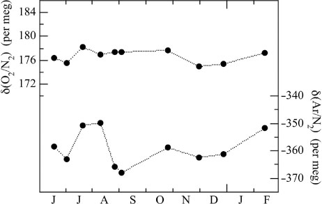
Fig. 8
Temporal changes of δ(O2/N2) and δ(Ar/N2) of the working standard air against the primary standard air.
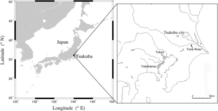
Fig. 9
Location of the city of Tsukuba, Japan.
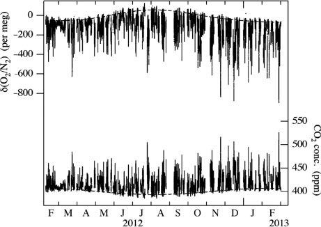
Fig. 10
Observational results of the atmospheric δ(O2/N2) and CO2 concentration at Tsukuba, Japan. The best-fitted curves consisting of two-harmonics and a linear trend to the daily maximum (minimum) values of the δ(O2/N2) (CO2 concentration) are also shown.
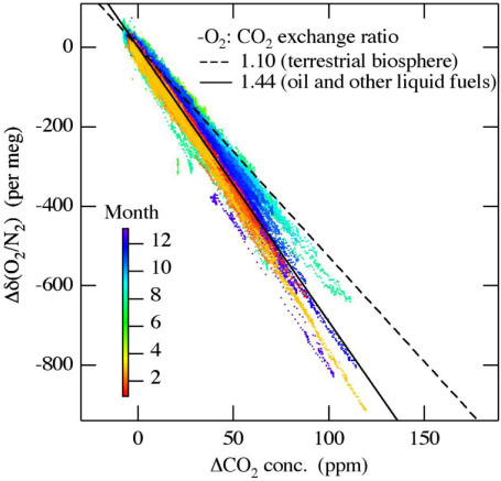
Fig. 11
Relationship between the δ(O2/N2) and the CO2 concentration shown in Fig. 10. Δδ(O2/N2) (ΔCO2) is the difference between the observed δ(O2/N2) (CO2) values and their best-fitted curve shown in Fig. 10. Colour bar denotes observation months. Dashed and solid black lines denote -O2: CO2 exchange ratio expected from the terrestrial biospheric activities and the combustion of oil and other liquid fuels, respectively.
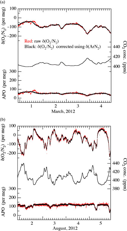
Fig. 12
δ(O2/N2), CO2 concentration and APO observed at Tsukuba, Japan on March 1–4 (a) and August 2–5 (b), 2012, after (black dots) and before (red dots) correcting for the fractionation due to thermal diffusion using the simultaneously observed δ(Ar/N2) values (see text).
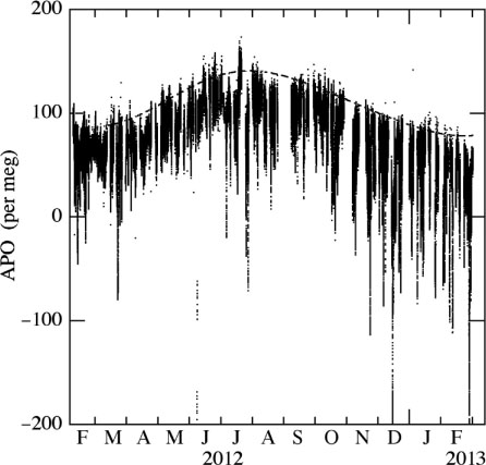
Fig. 13
Observational results of APO at Tsukuba, Japan. The best-fitted curve consisting of two-harmonics and a linear trend to the daily maximum values is also shown.
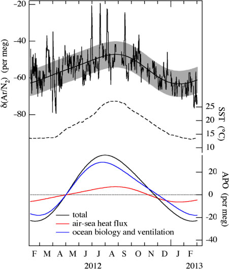
Fig. 14
24-hour running mean values of the δ(Ar/N2) observed at Tsukuba, Japan. The best-fitted curve consisting of two-harmonics and a linear trend to the data is also shown, and the shade around the fitted curve represents standard deviation of the observational data from the fitted curve (top). Sea surface temperature (SST) around Japan from NCEP NOMADS Meteorological Data Server (middle). Seasonal components of total APO, the APO driven by air–sea heat flux, and ocean biology and ventilation estimated from the observed APO and δ(Ar/N2) (see text; bottom).