
{ label needed for table-wrap[@id='UT0001'] }
Table 1. Chemical composition, mean diameter, and standard deviation of the eight lognormally distributed modes used for interactive simulations in this paper
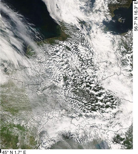
Fig. 1
Satellite image (true colour, MODIS-AQUA) of 25 April 2008.
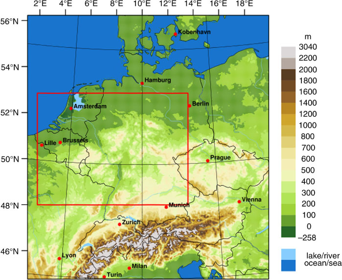
Fig. 2
Simulation domain and model orography. The red box indicates the convection domain.
{ label needed for table-wrap[@id='UT0002'] }
Table 2. The prescribed aerosol scenarios following Segal and Khain (2006)
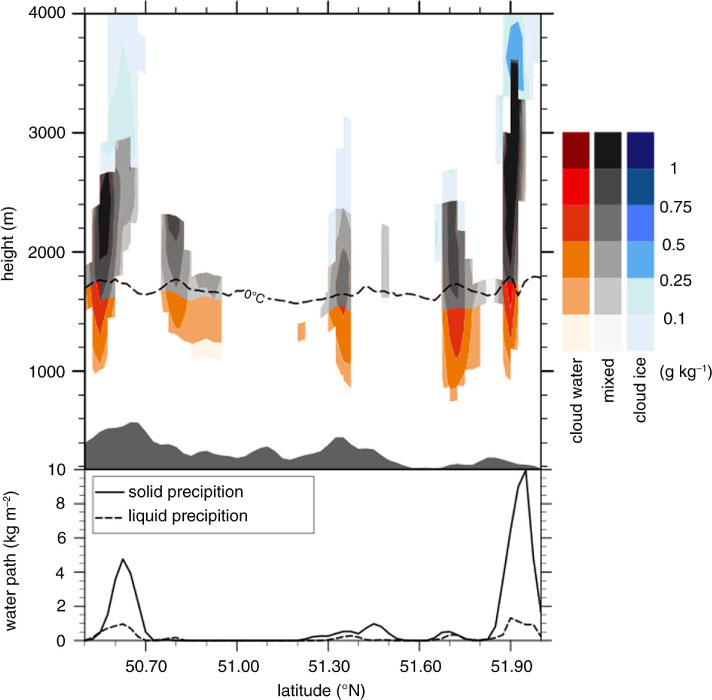
Fig. 3
Top: Cross-section for cloud water and ice content greater than 0.01 g kg−1 at 15 UTC. The position of the cross-section can be seen in Fig. 4b. Warm phase clouds have a red, mixed phase clouds a grey, and cold phase clouds a blue shading. The 0°C isotherm is shown as a dashed line. Bottom: Vertically integrated rain water content (dashed line) and vertically integrated snow and graupel content (solid line).
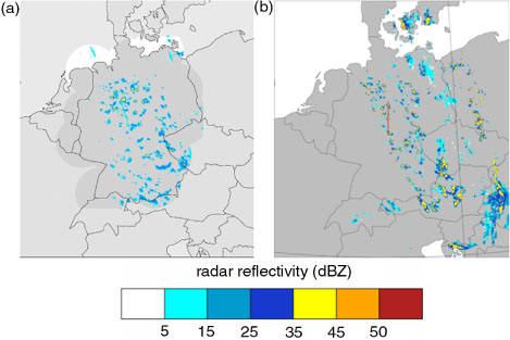
Fig. 4
(a) Measured radar composite (Seifert, 2009, personal correspondence), and (b) simulated radar reflectivity in dBZ for the interactive scenario at 850 hPa on 25 April 2008 15 UTC. The observations cover only a limited domain indicated by the grey (above land) and white (above sea)-shaded areas, whereas the model results are presented for the entire model domain. The red line indicates the cross-section from Fig. 3.
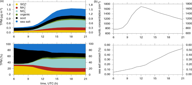
Fig. 5
(a) Temporal evolution of aerosol mass concentrations of the individual aerosol components averaged over the convection domain at the altitude of the cumulus clouds (≈850 hPa) during 25 April 2008 for the interactive scenario. (b) Corresponding total aerosol number concentration and sea salt number fraction.
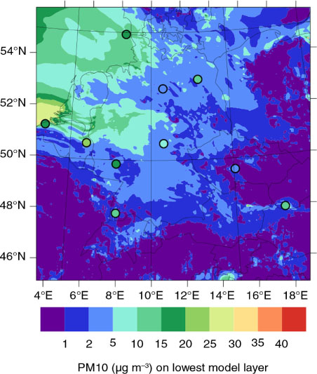
Fig. 6
Simulated PM10 concentration at 15 UTC on 25 April 2008. The model results are shaded, measured concentrations from EEA-AIRBASE EMEP stations are shown by coloured dots (EuropeanAIR quality dataBASE, http://airbase.eionet.europa.eu/).
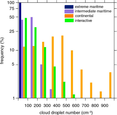
Fig. 7
Histogram of cloud droplet number concentration for grid points in the convection domain between 6 UTC and 21 UTC with cloud liquid water content greater zero.
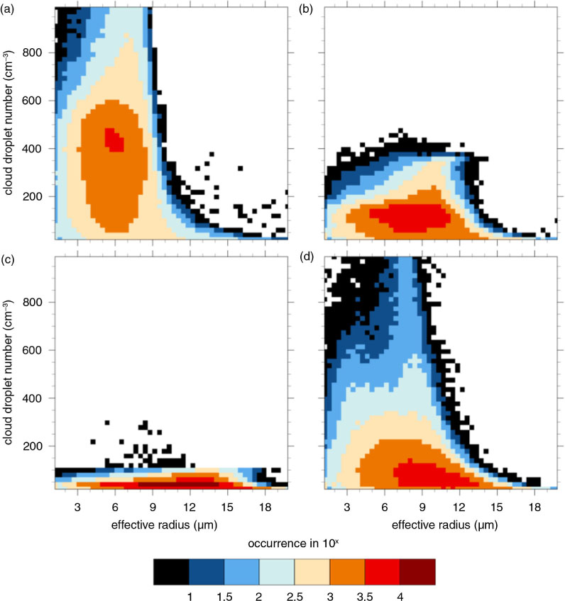
Fig. 8
Joint histograms of cloud properties for (a) continental, (b) intermediate maritime, (c) extreme maritime and (d) interactive scenario for grid points in the convection domain between 6 UTC and 21 UTC with cloud liquid water content greater zero.
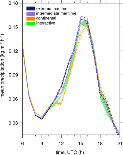
Fig. 9
Mean hourly precipitation rate within the convection domain of 25 April 2008 for four scenarios. The solid line is the mean value. The dashed lines indicate the standard deviation. The ensemble is generated as described in Section 3.1 and indicates the uncertainty due to the non-linearity of the atmospheric processes. As the interactive scenario has only three ensemble members, the spread is indicated by the shaded area.
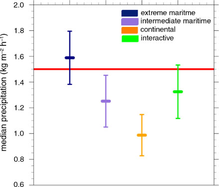
Fig. 10
Median accumulated precipitation at 58 EOBS-stations (Klok and Klein Tank, 2009) within the convection domain. The red line indicates the median of the measurements. The middle line gives the ensemble mean value. The top and bottom lines indicate the standard deviation. The ensemble is generated as described in Section 3.1 and indicates the uncertainty due to the non-linearity of the atmospheric processes.
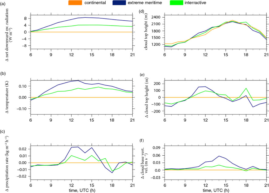
Fig. 11
Relative difference of extreme maritime scenario and interactive model run to the continental scenario in (a) net downward shortwave radiation at the surface, (b) temperatures of the lowest model layer, (c) hourly precipitation rate, (e) cloud top height, and (f) cloud base vertical velocity, (d) shows the total cloud top height. All variables are averaged over the convection domain.