
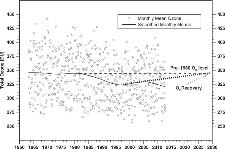
Fig. 1
Total ozone monthly means from the Dobson spectrophotometer measurements at Belsk in the period March 1963−December 2012. The solid line shows the long-term variability in the data by the LOWES smoother. Two dashed lines, horizontal line showing the pre-1980 ozone level and the sloped line, are shown for an estimation of the recovery time based on the ozone increase rate in the period 1997–2005.
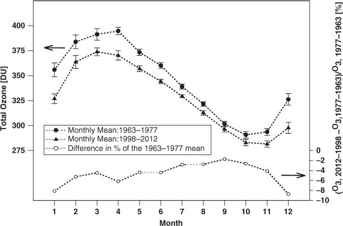
Fig. 2
The long-term total ozone monthly means for the first (1963–1977) and last (1998–2012) 15-yr period of the ozone observations at Belsk and the relative monthly differences between these means as a percent of the means in the former period.
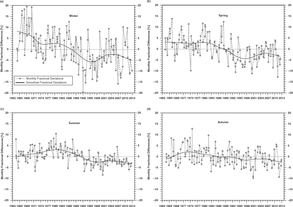
Fig. 3
The monthly differences of total ozone relative to the long-term (1963–2012) means as a percent of the long-term means: (a) winter – DJF; (b) spring – MAM; (c) summer – JJA and (d) autumn – SON.
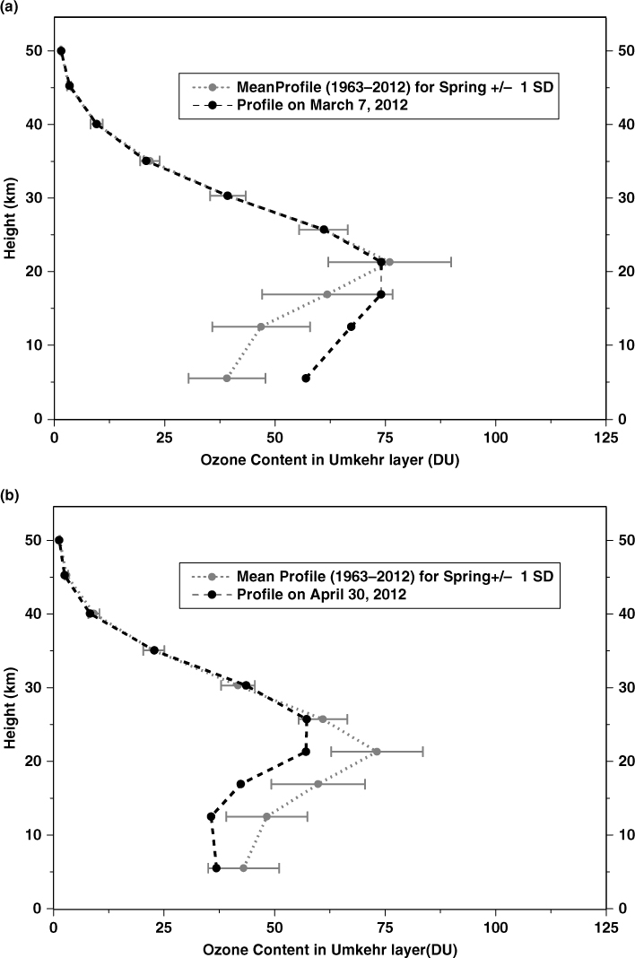
Fig. 4
Examples of the Umkehr ozone profiles superposed on the long-term (1963–2012) monthly mean profiles: (a) with a positive decline in the lower stratosphere – 7 March 2012 and (b) with a negative decline in the lower stratosphere – 30 April 2012.
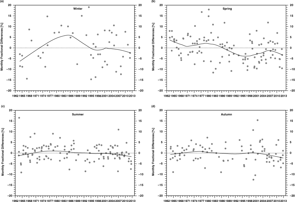
Fig. 5
The same as Fig. 3 but for the subset of the total ozone values taken only in days with the Umkehr observations.
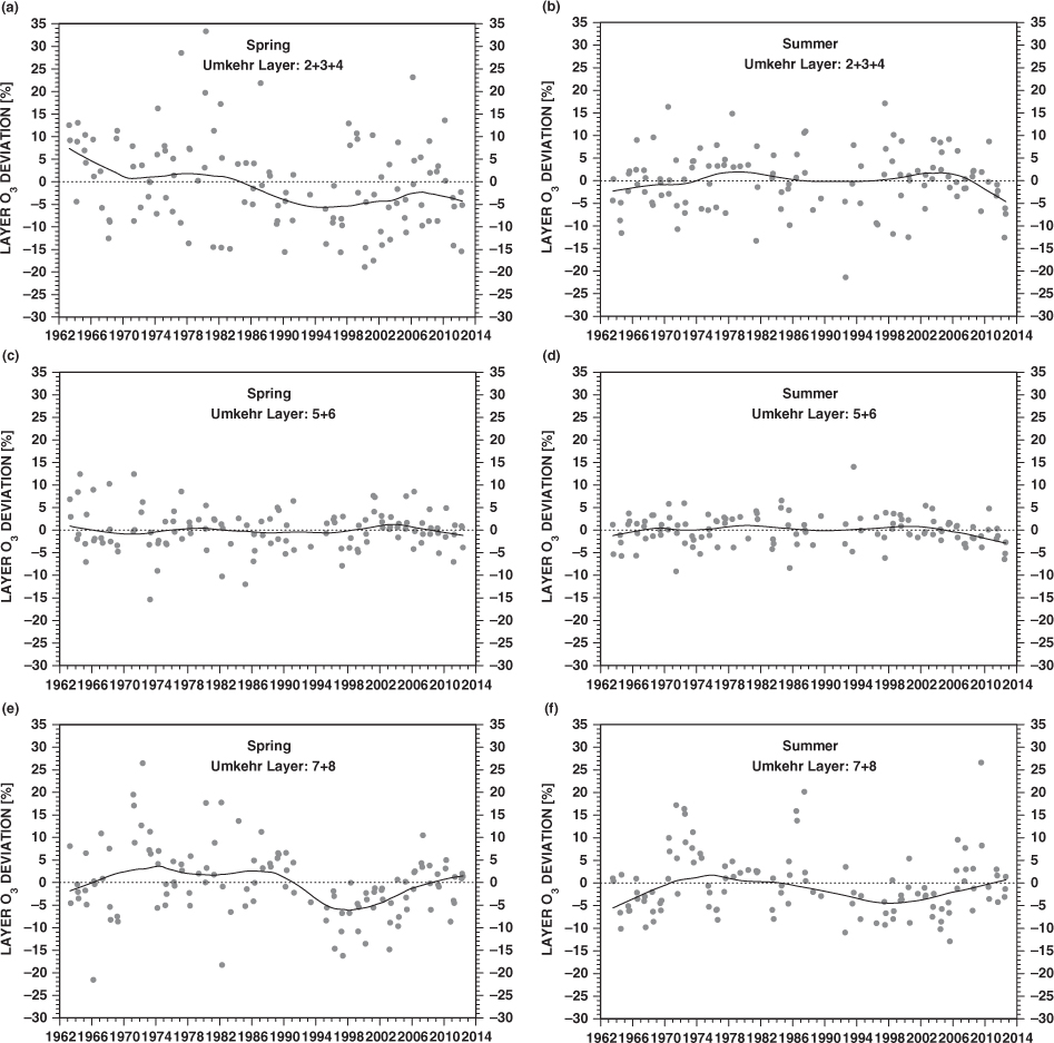
Fig. 6
The monthly differences of ozone content in the combined Umkehr layers in the period 1963–2012 relative to the long-term means for that period as a percent of the long-term means: spring (left-hand side), summer (right-hand side).
Table 1. The explanatory variables used in the study
http://www.cpc.noaa.gov/data/indices/qbo.u30.indexAO Indexhttp://www.cpc.ncep.noaa.gov/products/precip/CWlink/daily_ao∣_index/ao_index.htmlENSO indexhttp://www.cpc.ncep.noaa.gov/products/analysis_monitoring/en∣sostuff/detrend.nino34.ascii.txtEESC based on WMO Scenario A1_2010 mid-latitudes: mean age of air 3 yr., age of air-spectrum width 1.5 yrNASA Goddard Institute for Space Studies http://acdb-∣ext.gsfc.nasa.gov/Data_services/automailer/Penticton 2800 Hz Solar FluxNOAA National Geophysical Data Center
ftp://ftp.ngdc.noaa.gov/STP/SOLAR_DATA/SOLAR_RADIO/∣FLUX/Penticton_Adjusted/monthly/MONTHLY.ADJStratospheric aerosol optical depth at 550 nm – zonal mean for ~50°N latitudehttp://data.giss.nasa.gov/modelforce/strataer/Temperature at 50 hPa and 10 hPa levels, and the tropopause pressure interpolated from the gridded dataCDAS-NCEP/NCAR Reanalyses 4x daily 1948–2012 ∣ Annual Meteorological Statistics: http://nomad3.ncep.noaa.gov/cgi-bin/pdisp_6p_r1.sh
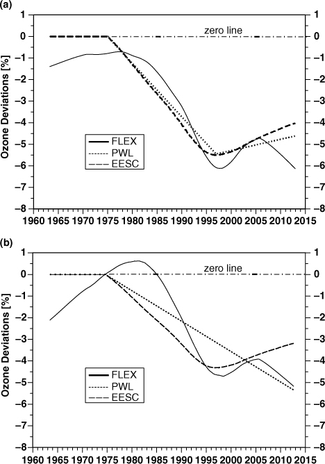
Fig. 7
The trend curves used in the examined models of the ozone variability (dashed – EESC, dotted – PWLT, solid – FLEX): (a) winter (DJF) total ozone, (b) summer (JJA) total ozone.
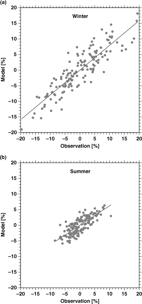
Fig. 8
The modelled monthly deviations of total ozone relative to the long-term (1963–2012) means as a percent of the long-term mean versus those from the observations. (a) winter (DJF), (b) summer (JJA). The straight line shows the standard least squares fit to the data.
Table 2
The trends by the examined trend models for the four seasons of the year and the year-round monthly total ozone values
Table 3. The same as Table 2 by the trends are for the ozone content in the selected combined Umkehr layers and for sum of the ozone content in all 10 layers (total ozone)
Table 4. The probability of appearance of the total ozone trend in the period 1997–2012 higher than that in the period 1975–1996 (Tr75–96<Tr97–12), the positive trends in the period 1997–2012 (Tr97–12>0), 1997–2005 (Tr97–05>0) and 2005–2012 (Tr05–12>0)
Table 5. The same as Table 4 but results are for the Umkehr total ozone and the ozone content in the joint neighbouring Umkehr layers: 2+3+4 – the lower stratosphere, 5+6 – the middle stratosphere, and 7+8 – the upper stratosphere