
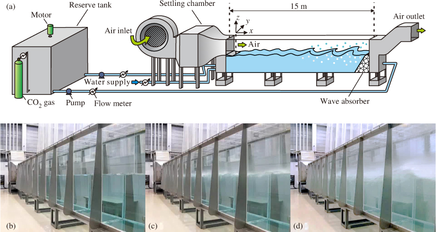
Fig. 1
(a) Schematic diagram of the high-speed wind-wave tank. (b), (c) and (d) are the photographs of wind waves at low, moderate and high wind speeds.
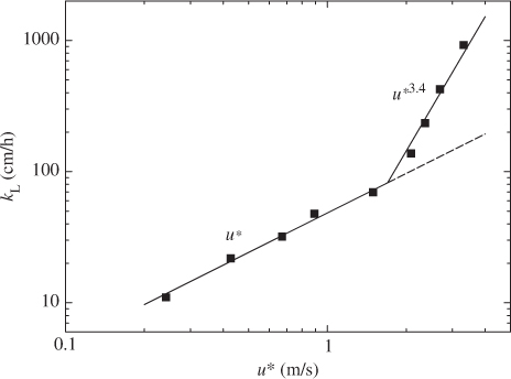
Fig. 2
Mass transfer velocity k L against air-friction velocity u*.
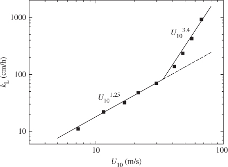
Fig. 3
Mass transfer velocity k L against wind speed at 10 m height U 10.
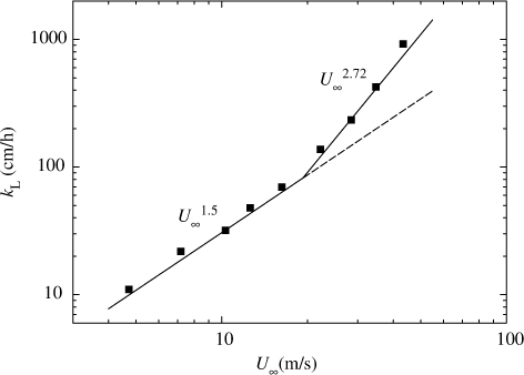
Fig. 4
Mass transfer velocity k L against free-stream wind speed U ∞.
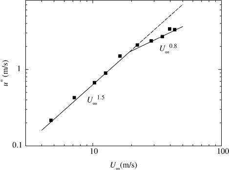
Fig. 5
Air-friction velocity u* against free-stream wind speed U ∞.
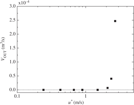
Fig. 6
Volume flux of dispersing droplets V OUT against air-friction velocity u*.
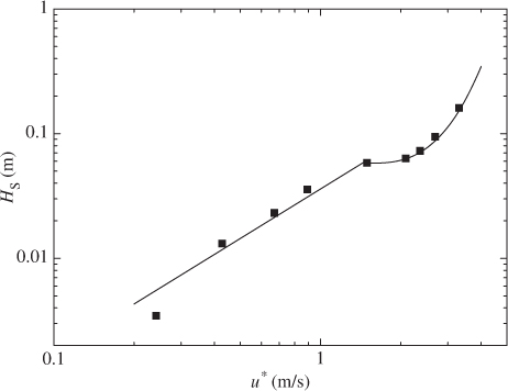
Fig. 7
Mean height of significant waves H s against air-friction velocity u*.
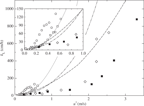
Fig. 8
Comparison of k L between laboratory and field measurements against u*. Data from this study (laboratory, CO2, solid squares), McGillis et al. (2001) (field, CO2, open squares), McGillis et al. (2004) (field, CO2, open triangles), Jacobs et al. (2002) (field, CO2, open circles), McNeil and D'Asaro (2007) (field, O2 and N2, open diamonds). A dashed line, a dotted line and a dashed-dotted line show the conventional k L correlation curves proposed by Wanninkhof (1992), Wanninkhof and McGillis (1999) and Wanninkhof et al. (2009) respectively.
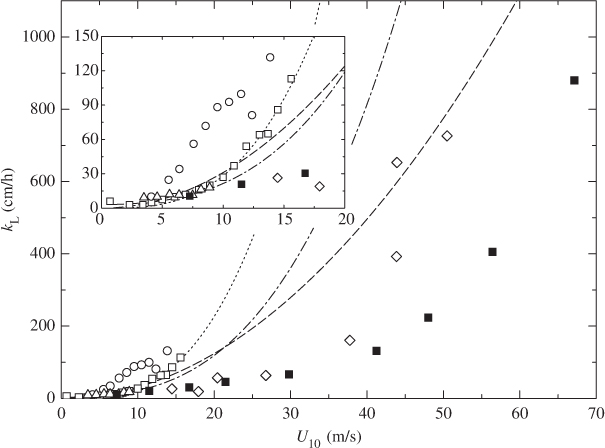
Fig. 9
Comparison of k L against U 10 between laboratory and field measurements. Symbols and lines as in Fig. 8.
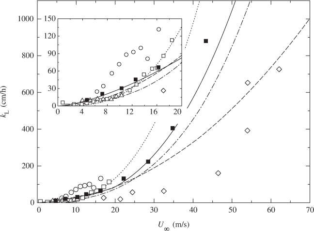
Fig. 10
Comparison of k L against U ∞ between laboratory and field measurements. Symbols and lines as in Fig. 8. A solid line shows the correlation curve of eq. (11) normalized to Sc=660 for the present laboratory measurements.