
Fig. 1
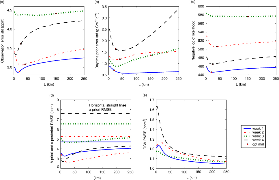
Hyperparameter estimation results using the Desroziers scheme. The estimations are conducted respectively for 4 weeks of June in 2007 with different correlation lengths Ls listed in the x-axis. We show the resulting hyperparameters: (a) optimal standard deviation (sd) of observation errors; (b) optimal sd of daytime prior flux errors. The criteria evaluated for these optimal hyperparameters are: (c) negative logarithm of the likelihood computed with optimal hyperparameters; (d) the root mean-square error (rmse) for the CO2 mole fraction simulations at all towers using a priori and a posteriori CO2 surface fluxes; (e) the GCV predictive mean-square error (pmse). The optimal correlation lengths bearing maximum likelihoods and the corresponding optimal sds are marked out by the circles in (a), (b) and (c).

Fig. 2
Inversion results with the optimal hyperparameter σ o, σ b and L (20 km) under the maximum likelihood (ML) criterion for the first week of June in 2007. The fluxes are in g C m−2 d−1. (a) Daytime inverted surface fluxes; (b) correction of the daytime inverted fluxes against the prior SiBcrop fluxes; (c) flux corrections of (b) normalised by σ b; (d) regions where the flux corrections of (b) are within one-sigma (indexed by 0) or out of one-sigma but within two-sigma (indexed by one).
Table 1. Values and standard deviations of the ML estimates for the observation error sd σ o in ppm, the daytime flux error sd σ b in g C m−2 d−1, and the Balgovind prior error correlation length L in kilometres
Week 12.89±0.1493.21±1.1320±6.77Week 23.08±0.1815.45±1.9940±13.6Week 3–––Week 43.62±0.2417.51±3.4825±7.90
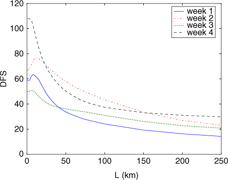
Fig. 3
Numbers of DFS with respect to correlation length L in prior flux errors for 4 weeks of June in 2007. Inversions are performed using optimal hyperparameters obtained by the Desroziers scheme. X-axis lists different correlation length Ls.
Table 2. Comparison between the total regional error budget of a priori fluxes (‘budget’ column) and the total regional flux correction by inversions (‘correction’ column) for the 4 weeks of June in 2007
week 120227201week 240742601week 31502546674week 425658621
[i] The optimal hyperparameters obtained by the Desroziers method (marked out by the circles in Fig. 1a and b) are used for this comparison.