
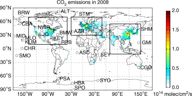
Fig. 1
Spatial distribution of FF CO2 emissions for 2008 and the locations of 24 GLOBALVIEW-CO2 sites (circles); the black boxes indicate the definition of three regions: North America (NA; 10° to 70°N, −140° to −40°E), Europe (EU; 30° to 70°N, −30° to 50°E) and Asia (AS; −11° to 55°N, 70° to 150°E).
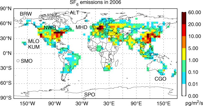
Fig. 2
Spatial distribution of SF6 emissions for 2006 and the locations of 9 NOAA ESRL SF6 observation sites (circles).
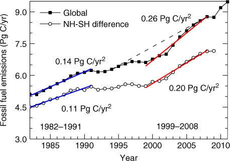
Fig. 3
Global total (filled squares) and IHD (open circles) of FF emissions during 1982–2011. The growth rates of FF emissions during 1982–1991 and 1999–2008 are listed in the figure. The dashed lines are linear interpolated global FF emissions from 1994 to 2008.
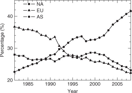
Fig. 4
The share of FF emissions from NA, EU and AS (regions defined in Fig. 1) to the global total FF CO2 emissions during 1982–2008.
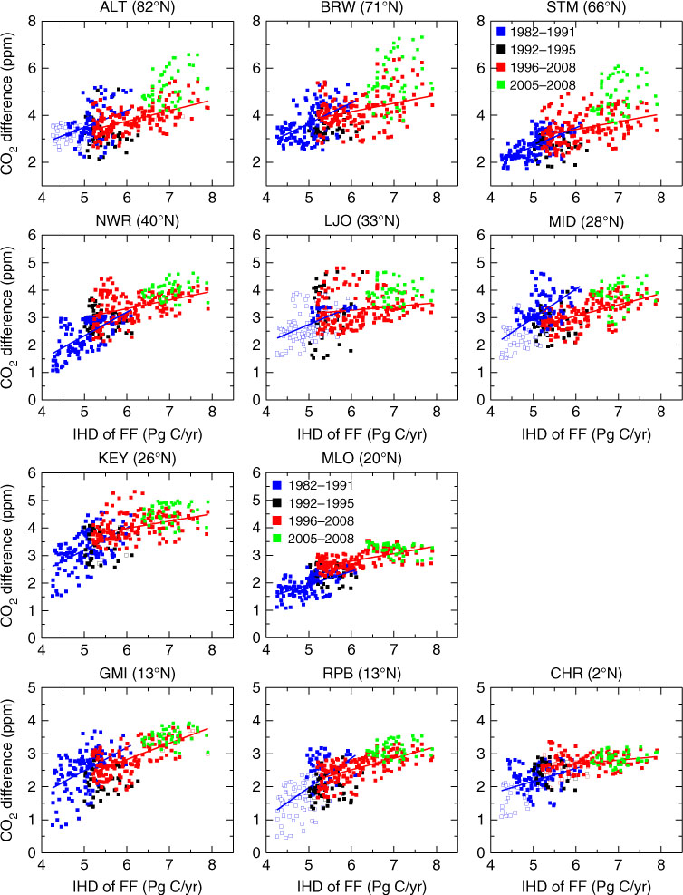
Fig. 5
The scatter plots between the IHD of CO2 and IHD of FF emissions for 11 sites in the NH. Blue and red lines are linear regression results for 1982–1991 and 1996–2008, respectively. The data for 1992–1995 are shown in black. The open squares represent the extended data for each site in GLOBALVIEW-CO2. The green squares are the results of corrected IHD of CO2 for 2005–2008 which eliminate the influence of the change in the spatial distribution of FF emissions.
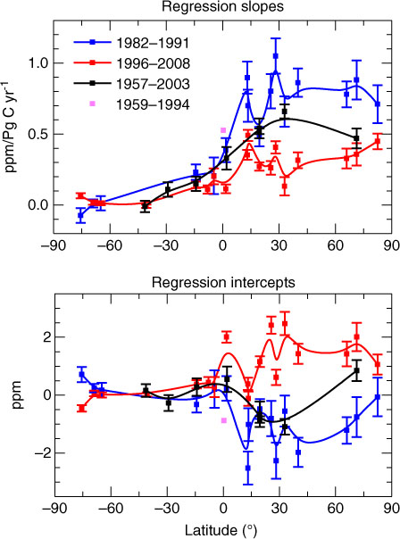
Fig. 6
Regression slopes and intercepts between the IHD of CO2 and IHD of FF emissions plotted as a function of latitude. The error bars represent ±1σ uncertainties of slopes and intercepts. The solid lines are results smoothed by a B-spline fit. The blue and red lines are results for 1982–1991 and 1996–2008 in this study. The black line is result from Keeling et al. (2011). The pink point is result from Fan et al. (1999).
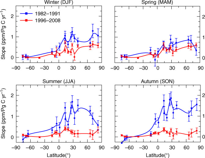
Fig. 7
Regression slopes between the IHD of CO2 and IHD of FF emissions in each season for 1982–1991 (blue) and 1996–2008 (red).
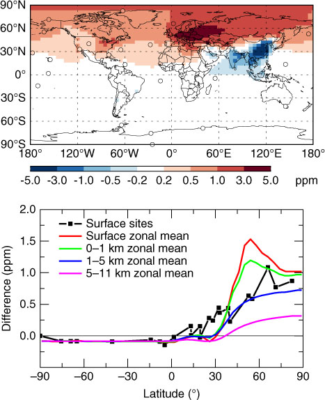
Fig. 8
The average difference in atmospheric CO2 between the sensitivity and standard simulation (sensitivity minus standard) for 2005–2008. Upper panel: the spatial distribution of the difference in surface CO2 (circles indicate the location of surface sites in this study); Bottom panel: the zonal-mean difference of CO2 at the surface, 0–1 km, 1–5 km and 5–11 km.
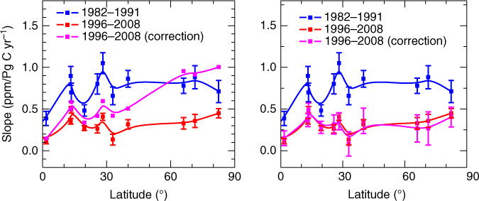
Fig. 9
Comparisons of the corrected regression slopes with those shown in Fig. 6 (blue and red lines) in the NH. Left panel: regression slopes using the corrected IHD of CO2 which eliminate the influence of the change in distribution of FF emissions (pink line); Right panel: regression slopes using the linearly interpolated global FF emissions from 1994 to 2008 as shown in Fig. 3 (pink line).
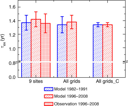
Fig. 10
Decadal averages of observed and simulated τ ex for 1982–1991 and 1996–2008 for three cases with different calculation of hemispheric-mean mixing ratios and emission scenarios: (1) ‘9 sites’ case: average of 6 sites in the NH and 3 sites in the SH, EDGAR4.0/Levin; (2) ‘All grids’ case: average of all surface NH and SH grids, EDGAR4.0/Levin; and (3) ‘All grids_C’ case: average of all surface NH and SH grids, EDGAR_Y1980.
Table 1. The biases and correlations between monthly simulated and observed SF6 at 9 NOAA observation sites during 1996–2008
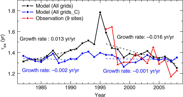
Fig. 11
Annual observed and simulated τ ex (solid lines) in the three cases in Fig. 10. The dashed lines are the linear trends of simulated τ ex for 1982–1991 and 1996–2008.
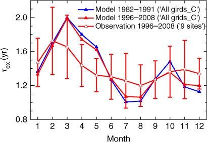
Fig. 12
Seasonal variation of observed (‘9 sites’ case) and simulated (‘All grids_C’ case) τ ex for 1982–1991 and 1996–2008.
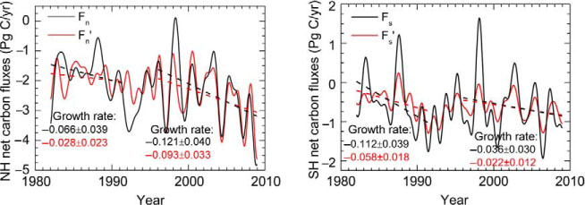
Fig. 13
Monthly net carbon fluxes (seasonally adjusted) in the NH (left panel) and SH (right panel). Black lines are the originally calculated fluxes with the two-box model (F n and F s ). Red lines are EVI-filtered fluxes after removal of the ENSO-Volcano related IAV in the original calculated fluxes (F n ′ and F s ′). The dashed lines are the linear trends for 1982–1991 and 1996–2008. Mean values and ±2σ uncertainties of the growth rate for each period are listed in the figure in Pg C/yr2. Negative values indicate net carbon sink.
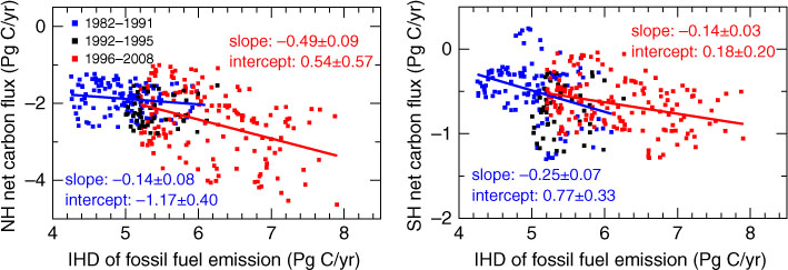
Fig. 14
Linear regressions between the IHD of net carbon fluxes (left panel: original calculation; right panel: EVI-filtered) and IHD of FF emissions during 1982–1991(blue) and 1996–2008 (red). The data for 1992–1995 are shown in black.
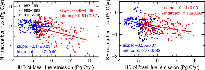
Fig. 15
Linear regressions between the EVI-filtered hemispheric net carbon fluxes (F n ′ and F s ′) and the IHD of FF emissions for 1982–1991(blue) and 1996–2008 (red). The data for 1992–1995 are shown in black. The left panel shows the NH data and the right panel shows the SH data.