
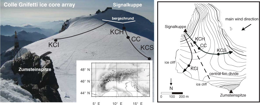
Fig. 1
Geographical situation of the Colle Gnifetti saddle in the Monte Rosa summit range (45° 56′ N, 7° 52′ E, 4450 m asl) with the position of the four ice cores within the north flank area. Approximate surface flow lines are shown by black arrows along with the surface topography displayed by contour lines at 20 m altitude spacing.
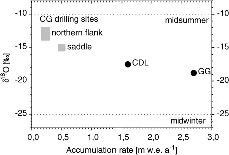
Fig. 2
Mean δ18O levels in recent firn and ice records of the Monte Rosa region versus mean snow accumulation rate. Grey rectangles at Colle Gnifetti mark the δ18O and accumulation rate ranges within the north flank and near saddle areas. CDL and GG denote cores drilled at the relatively wind protected sites Colle del Lys (B. Stenni, pers. communication) and Grenzgletscher (Eichler et al., 2000). Mid-winter and summer levels indicate the typical overall range of the raw datasets.
Table 1
Glaciological features of the evaluated Colle Gnifetti ice cores
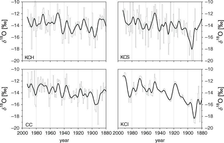
Fig. 3
Colle Gnifetti δ18O time series over the last 120 yr displayed in nominal annual resolution (see text) with trends highlighted by decadal Gaussian smoothing. Note the relatively small effect of this low pass filter on the KCI δ18O record having been smoothed strongly already by isotope diffusion.
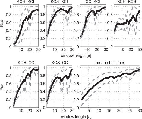
Fig. 4
Binned correlation coefficient R bin over the common period 1981 to 1880 of each pair of the Colle Gnifetti δ18O time series as a function of binning window length (black lines). The grey dashed lines indicate the 90% confidence intervals obtained from multiple runs with varying starting point of the binning. Lower panel, right side: The mean value calculated for R bin from all pairs of δ18O time series (1981–1880), plotted as a function of binning window length. Grey dashed curves indicate one standard deviation around the mean. For details on the binned correlation calculation, see Supplementary Material.
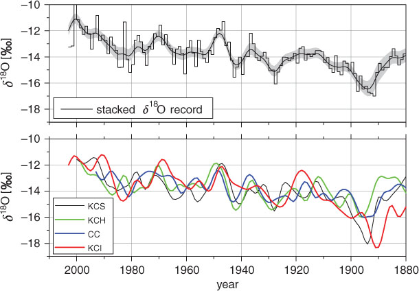
Fig. 5
Upper panel: composite (stacked) δ18O record from four Colle Gnifetti cores smoothed by decadal Gaussian filter (black line) with bootstrap uncertainty estimate displayed as grey band. Lower panel: Same as upper panel but for the individual δ18O records.
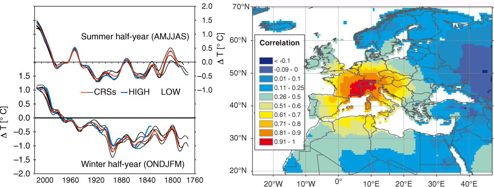
Fig. 6
Left panel: 30-yr Gaussian low pass filter of the 1760–2007 instrumental temperature series compiled for the 5 subregions of the Greater Alpine Region HISTALP database (Auer et al., 2007). CRSs refers to the four low elevation subregions, LOW to low elevation mean and HIGH to high elevation mean. The slightly larger spatial heterogeneity in the early instrumental period (prior to 1850) than today is rather an artefact of still existing homogeneity problems than an expression of real climate patterns. Right panel: Spatial coherence of air temperature in Europe shown by the grid-point correlation (Pearson correlation coefficient) for 1901–2002 of the Climatic Research Unit (University of East Anglia, UK) temperature series versus the Colle Gnifetti grid-point (see text for data source).
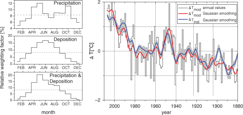
Fig. 7
Left panel: Monthly weighting factors for precipitation (top), net snow deposition probability (middle) and both combined (bottom) used for establishing the modified instrumental temperature series ΔT mod with annual averages indicated by dashed lines. Right panel: Comparison of ΔT mod versus the original temperature record ΔT inst; both anomalies refer to the 2007–1880 mean. The uncertainty associated with the original instrumental temperature record is indicated by the grey band (see text).
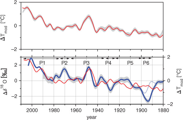
Fig. 8
Intercomparison of decadal changes of the modified instrumental temperature ΔT mod (upper panel, red line) with stacked δ18O record (lower panel blue line). All data are smoothed by decadal Gaussian filtering and refer to deviations from the 2003–1880 mean. Grey bands indicate the estimated uncertainty ranges, which are adopted for ΔT mod without change from ΔT inst (Fig. 7) and from the bootstrap uncertainty of δ18O shown in Fig. 5. The dotted blue line refers to the isotope stack corrected for the outlier around 1890 (see text). The periods marked with P1 to P6 are discussed in the text.
Table 2
Overview on climatologic findings from the HISTALP high elevation database during misfit and non-misfit periods between the δ18O and instrumental temperature records marked in Fig. 8
[i] The ratings ‘high’ and ‘low’ refer to decadal deviations above and below the robust trend, which was extracted by SSA. The amplitude of the largest decadal feature (Gaussian smoothing) within the respective period is quantified to aid relative comparison. For sunshine duration, the relative increase/decrease is given in per cent of the overall 2000–1901 mean. If a clear indication for high or low is missing, an entry is omitted (‘–’).
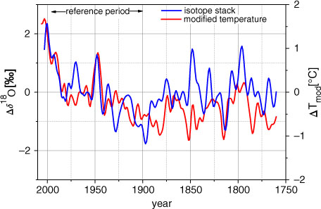
Fig. 9
Comparison of the composite δ18O record (red line) with instrumental temperature data (blue line) as in Fig. 8 but extended to the full instrumental period back to 1760. Note that the outliner corrected δ18O record is used. Data are shown as deviations from the 2000–1901 mean.
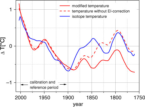
Fig. 10
Centennial scale trends of temperature anomalies relative to the 2000–1901 mean derived by the first component of Singular Spectrum Analysis (embedding length of 1/5 of the entire time series length). Blue line: ΔT based on the outlier corrected δ18O stack adopting an isotope/temperature sensitivity of 1.6‰/°C, solid red line: modified instrumental temperature ΔT mod based on Auer et al., 2007, dashed red line: high Alpine instrumental summer temperature without the early instrumental correction (Böhm et al., 2001; Böhm et al., 2010).