
Table 1
Summary of cloud properties for clouds>300 m in width. Maximum cloud drop number concentrations and leg mean N aerosol (#/cm−3) and N acc (#/cm−3), one standard deviation in parenthesis, are from Table 2 of (Lu et al., 2008). The (Lu et al., 2008) are for full legs and have not been sorted for clouds>300 m in width. They are included for reference only. Two values are reported for L1 corresponding to two separate UTC time periods. Though (Lu et al., 2008) reports high leg mean N aerosol for L2, the large standard deviation is the result of sampling a power plant plume (17:17 to 18:00 UTC) during an otherwise relatively clean flight. Values for average PDI cloud drop number concentration (CDNC) include data from all non-precipitating clouds greater than 300 m in width. For L2, two clouds sampled had peak CDNC values greater than 1000. With these two clouds excluded the maximum PDI CDNC is 983 cm−3
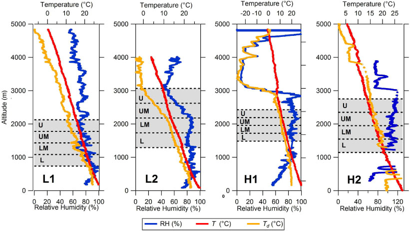
Fig. 1
Out-of-cloud atmospheric soundings. Vertical soundings for four full flights L1 (2006-Aug-26), L2 (2006-Sept-11), H1 (2006-Sept-08) and H2 (2006-Sept-15). Note that RH measurement problems occurred during large portions of the sounding for H2 (i.e. values above 100%). Grey shaded areas represent cloud layers (from lowest observed cloud base to highest observed cloud top) for each research flight. Approximate altitudes for cloud regions, lower (L), lower middle (LM), upper middle (UM) and upper (U) for each flight are separated by dotted lines.
Table 2
Full flight Wilcoxon ranked-sum test results for α, α weighted D v 3/D va 3 values and α weighted N/N a for full clouds. Each cloud region is compared to the others; that is, all of the D v 3/D va 3 data included in the Lower region of cloud is compared to all of the D v 3/D va 3 data in the Lower-Middle region of cloud and so on. Comparisons that result in statistically significant values, with p<0.01 are boldfaced. Six of the seven statistically significant comparisons are such that D v 3/D va 3 decreases with increasing height. A lack of data hampers comparisons of the Lower-Middle region with other levels for H2, and of the Upper Middle region with other levels for L2
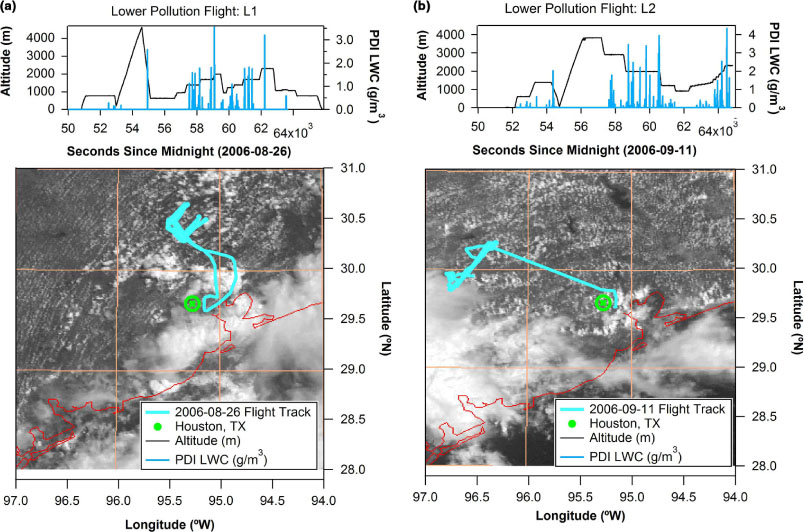
Fig. 2
Research flight paths and GOES-East imagery for lower pollution days. Flight paths and altitude and LWC profiles for (a) L1 and 1-km GOES-East image at 1600 UTC and (b) L2 and the 1-km GOES-East image at 1700 UTC. The coastline is represented by the red line and the location of Houston, Texas, is shown for reference.
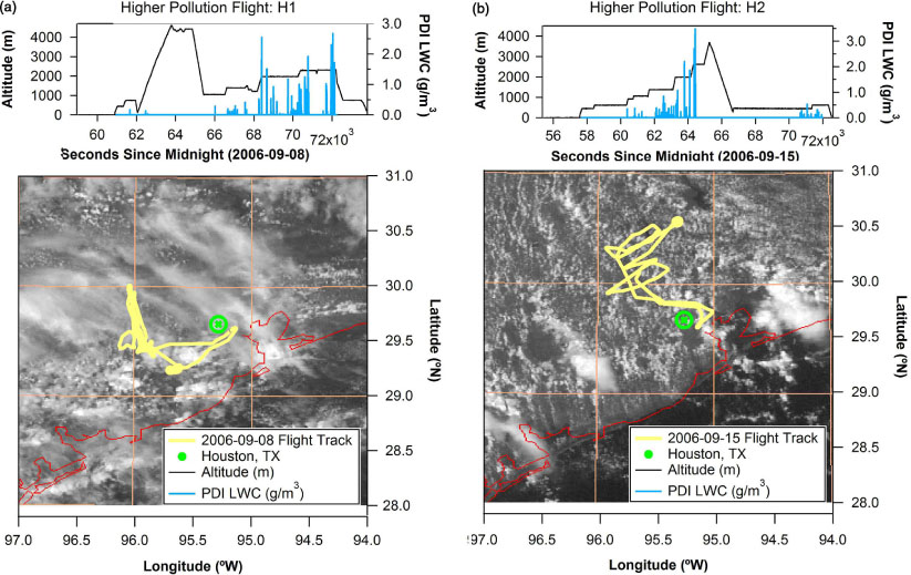
Fig. 3
Research flight paths and GOES-East imagery for higher pollution days. Flight paths and altitude and LWC profiles for (a) H1 and the 1-km GOES-East image at 1900 and (b) H2 and the 1-km GOES-East image at 1730. The coastline is represented by the red line and the location of Houston, Texas, is shown for reference.
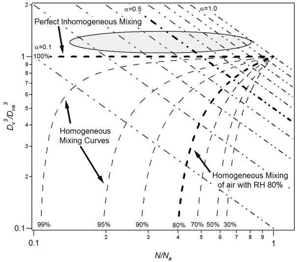
Fig. 4
Entrainment mixing diagram. Dashed lines represent the relationship between and N/N a during homogeneous mixing of air at various relative humidities. Bold dashed lines highlight mixing with air of 100 and 80% (the average ambient RH for the four flights included in study). The 100% RH homogeneous mixing line is the same as the inhomogeneous mixing line. Dash-dotted lines represent the dilution ratio, α=LWC/LWCa, where LWCa is the adiabatic liquid water content. α is plotted at 0.1 intervals from α=1 to α=0.1. Values in the region of the shaded oval may result if the chosen reference N a is too small for a particular cloud sample or if collision-coalescence is active. Note that collision-coalescence cannot yield samples with α>1, but this could happen if drops sediment into a sample volume from higher parts of cloud.
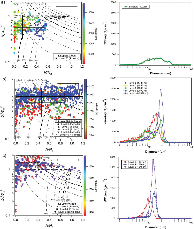
Fig. 5
1-Hz data plotted as a function of altitude and corresponding average DSD for each level (coloured markers and lines based on altitude) for (a) upper cloud, (b) lower-middle cloud and (c) lower cloud with 2-D box and whiskers representing 95, 75, median, 25 and 5 percentiles of all levels.
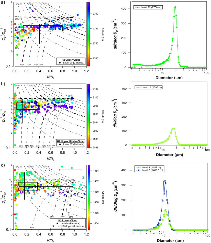
Fig. 6
1-Hz data plotted as a function of altitude (coloured markers) and corresponding average DSD for each level and individual clouds (coloured lines based on altitude) for (a) upper cloud, (b) upper-middle cloud and (c) lower cloud with 2-D box and whiskers representing 95, 75, median, 25 and 5 percentiles of all levels.
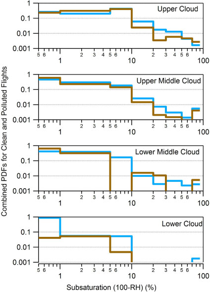
Fig. 7
PDF of relative humidity mixing wedges. Vertical profiles of turbulence quantities for individual flights. Combined histograms for lower pollution flights, L1 and L2 (blue curves), and higher pollution flights, H1 and H2 (brown curves). Data are first binned by relative humidity according to RH curves presented on mixing diagrams, with bins defined for RH 10–30%, 30–50%, 50–70%, 70–80%, 80–90% 90–95%, 95–99% and 99–100% (although the upper limit is plotted as 99.5%). The 99–100% humidity range would contain parcels that experienced perfect inhomogeneous mixing. The bins are then weighted to accommodate the differences in bin widths. Finally, sub-saturation is calculated for each bin by taking 100-RH for each of the bin boundaries. Such that a RH bin for 99–95% has a sub-saturation of 1–5%. This allows us to look at the 99–90% humidity range in more detail. Number counts for 10–30% bin represent data with N/N a values less than 1.2 or values less than 0.1. Data with greater than 1 are not shown.
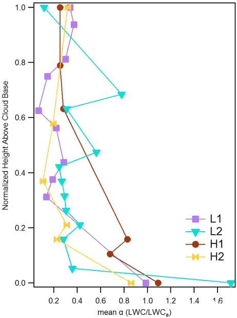
Fig. 8
Vertical profiles of α. Vertical profiles of adiabaticity α=LWC/LWCa for L1, L2, H1, and H2 as a function of normalised height above cloud base.
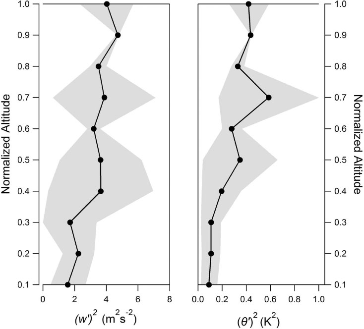
Fig. 9
Vertical profiles of turbulence quantities for individual flights. Vertical profiles of (a) fluctuations in vertical velocity, and (b) fluctuations of potential temperature, . Means across all four flights (L1, L2, H1 and H2) are calculated and one standard deviation is shown in grey for each normalised altitude bin.
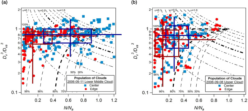
Fig. 10
Mixing diagrams displaying edge and centre data. Five-hertz cloud edge and centre samples for (a) the lower-middle region for L2, and (b) the upper region of H1. Edges for all levels are red circles, centres for all levels are blue squares with 2-D box and whiskers representing 95, 75, median, 25 and 5 percentiles of all levels.
Table 3. Full flight Wilcoxon ranked-sum test results for α weighted N/N a values for cloud centres and edges. Cloud edges and cloud centres for each cloud region are compared using the Wilcoxon signed-rank-sum test. Comparisons that result in statistically significant values, with p<0.01 are boldfaced
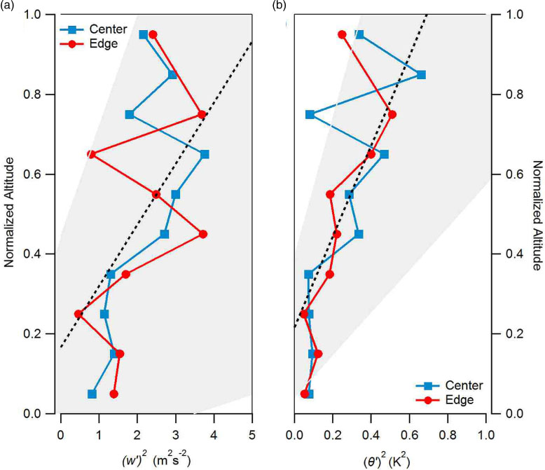
Fig. 11
Vertical profiles for centres and edges. Data for (a) fluctuations in vertical velocity, and (b) fluctuations of potential temperature, . Blue curves with square markers represent data from cloud centres for L1, L2, H1 and H2. Red curves with circle markers represent data from cloud edges for L1, L2, H1 and H2. Linear regressions for composites of all days, including both centre and edges (black dashed lines) and 95% confidence intervals for slopes are also represented (shaded area) showing the increase in turbulent quantities with height.