Have a personal or library account? Click to login
Analysis and evolution of air quality monitoring networks using combined statistical information indexes Cover

Analysis and evolution of air quality monitoring networks using combined statistical information indexes

Open Access
|Jan 2013

Figures & Tables

Fig. 1

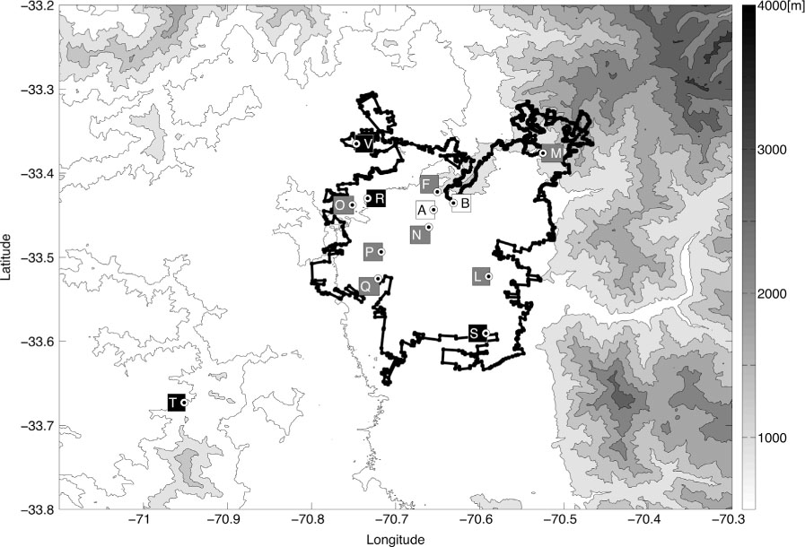
Location of monitoring stations in Santiago's air quality network since the 1980's (for details see text). The symbols correspond to the names of the stations A: Gotuzzo, B: Providencia (not used in this study, in white), F: Independencia, L: La Florida, M: Las Condes, N: Parque O'Higgins, O: Pudahuel, P: Cerrillos, Q: El Bosque (seven stations continuously working on the period 1997–2008, in grey), R: Cerro Navia, S: Puente Alto, T: Talagante, V: Quilicura (four more stations added on the period 2009–2010, in black). The limit of the current urban area is indicated by a heavy line. Main topographic features of the Santiago basin are also shown.

Table 1

Description of the air quality monitoring stations belonging over time to Santiago's monitoring network and the two periods of data used in this study.

Period and data usedLonLatHeightCharNameWSm a.s.l.TypeWorkingNot usedAGotuzzo70 65533 444576Commerce/services1988–1997BProvidencia70 63133 436592Close to main road/medium income1988–20022009–2010 (PM10, PM2.5, O3)1997–2008 (CO, PM10, O3, SO2)FIndependencia70 64933 419565Commerce/servicesSince 1988LLa Florida70 58633 513594Residential/low-medium incomeSince 1997MLas Condes70 52333 374775Residential/high incomeSince 1988NP. O'Higgins70 65833 461545In a park/close to highwaySince 1988OPudahuel70 74833 435494Residential/low incomeSince 1997PCerrillos70 71333 493511Residential/industrialSince 1997QEl Bosque70 66433 544582Residential/industrialSince 1997RCerro Navia70 73333 430498Residential/low incomeSince 2008SPuente Alto70 59333 591680Residential/low incomeSince 2009TTalagante70 95133 673401RuralSince 2009VQuilicura70 74733 365489Residential/low-medium incomeSince 2009
Table 2

Relative quadratic error in percentage using different statistical models for fitting the 1997–2008 data for 7 stations and 4 measured species and for the 2009–2010 data for 11 stations and 3 measured species.
NormalLog-normalGammaAllSWAllSWAllSWFor fitting the 1997–2008 hourly dataCO26.924.118.114.923.910.95.178.074.66O39.7610.58.9911.119.78.873.9310.52.06PM1010.56.468.961.871.503.940.630.411.17SO237.142.726.041.140.230.521.024.212.7For fitting the 2009–2010 hourly dataPM1016.37.638.551.781.083.382.250.701.06PM2.59.844.699.591.361.492.290.710.480.95O310.912.66.799.8116.96.893.859.783.30

[i] All data (All), segregated by summer (S: Dec, Jan, Feb) or winter (W: Jun, Jul, Aug) months.

Fig. 2

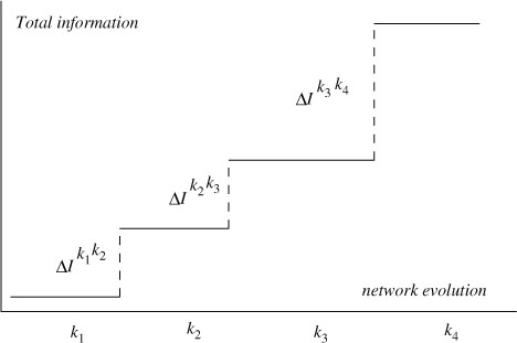
Schematic evolution of the total information of the network.

Table 3

Main statistics (mean, standard deviation and maximum) for each of the 7 monitoring stations working during the period 1997–2008 based on hourly averages during all the year (All), summer (S: Dec, Jan, Feb) and winter (W: Jun, Jul, Aug).

SpeciesFLMNOPQCO (ppb)All1.21.20.71.61.11.41.21.11.20.51.71.41.41.35.562.88.68.86.76.9S0.50.60.40.60.40.50.60.40.40.20.50.30.50.54.45.11.95.74.146.7W1.81.91.02.21.81.91.91.21.40.61.91.81.61.65.562.88.68.86.76.9O3 (ppb)All19.621.224.923.119.020.120.317.020.024.418.615.916.516.3718210678646966S23.327.133.427.223.324.724.418.421.727.919.316.617.017.2718210678646966W12.412.513.714.911.812.612.911.413.413.813.911.612.311.6718210678646966PM10 (µg/m3N)All72.180.956.774.277.875.980.343.553.836.750.658.452.754.9244309197288359293312S57.768.554.357.762.664.466.528.234.029.130.836.838.233.7239309196286358293290W88.394.457.992.695.990.994.752.667.243.261.973.663.667.8244309197288359293312SO2 (ppm)All4.974.463.435.024.14.965.053.43.32.13.72.73.43.822231423162127S4.03.63.03.83.23.84.32.62.81.92.82.02.53.622231423162127W6.35.23.96.45.16.55.94.03.62.34.33.13.94.022231423162127
Table 4

Main statistics (mean, standard deviation and maximum) for each of the 11 monitoring stations working during the period 2009–2010 based on hourly averages during all the year (All), summer (S: Dec, Jan, Feb) and winter (W: Jun, Jul, Aug).

SpeciesFLMNOPQRSTVO3All17.018.419.221.915.218.616.316.020.117.116.1(ppb)16.018.220.417.014.615.515.014.916.511.715.56673886959646060655163S21.525.328.026.021.024.321.821.325.218.622.117.820.524.118.016.016.616.915.917.611.716.76673886959646060655163W8.69.48.813.08.210.79.08.212.312.68.08.59.69.210.38.59.28.28.311.09.98.96268676754636058645061PM10 (µg/m3N)All50.157.145.755.848.358.961.952.349.537.473.322.824.222.126.523.228.527.424.821.420.539.2161215143206244199210292158142285S50.157.145.755.848.358.961.952.349.537.473.322.824.222.126.523.228.527.424.821.420.539.2161215143206244199210292158142285W69.379.146.880.781.574.979.488.255.451.783.336.554.629.749.058.944.353.965.233.534.855.5174268146234271204248295164156289PM2.5 (µg/m3N)All26.527.521.627.427.127.928.528.624.7320.427.014.716.112.117.822.219.521.125.914.416.318.5779066961361081271627988104S20.424.820.421.420.019.721.918.120.714.121.29.212.210.410.810.69.811.110.110.29.511.660866692136104100141778798W35.133.523.837.339.939.937.844.730.031.235.916.719.214.221.329.924.227.435.117.220.622.1779066961361081271627988104
Table 5

Percentage of available hourly data considering 7 stations (period 1997–2008) and 11 stations (period 2009–2010) for all years and months (All), summer (S: Dec, Jan, Feb) and winter (W: Jun, Jul, Aug).
SpeciesAllSWPeriod 1997–2008CO% original data959298% after filtering705287O3% original data969497% after filtering687955PM10% original data969499% after filtering949394SO2% original data919092% after filtering706278Period 2009–2010PM10% original data989999% after filtering969895PM2.5% original data989899% after filtering969794O3% original data939390% after filtering798672
Fig. 3

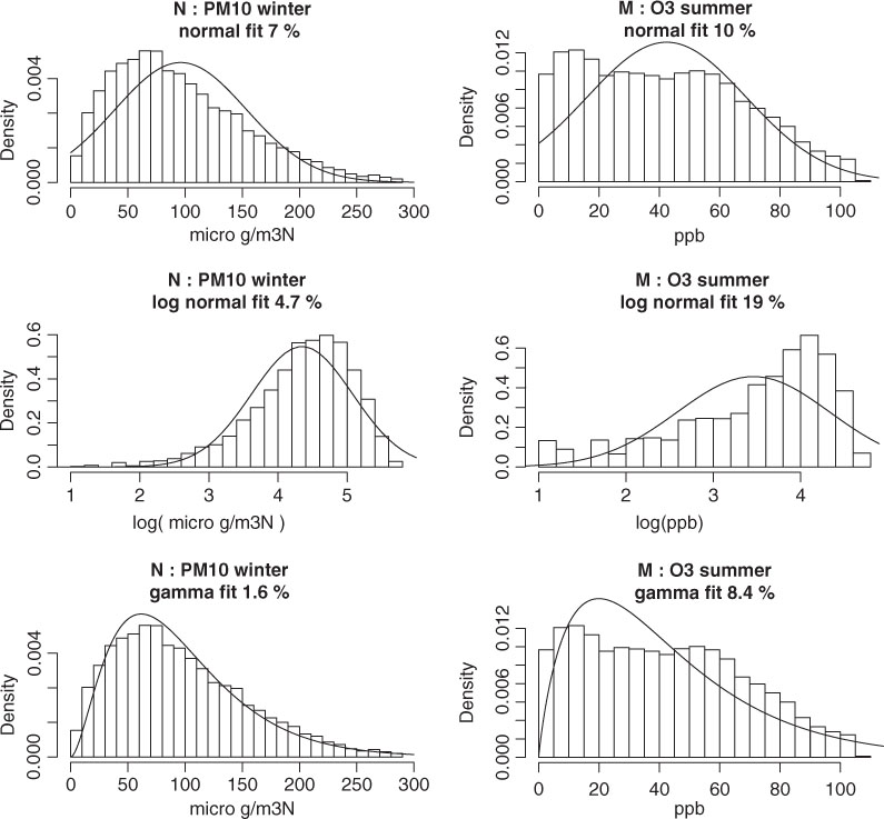
Example of some statistical fitting. PM10 in winter for station N and O3 for stations M for normal (top line), log-normal (middle line) and gamma (bottom line) fitting. The relative quadratic error is indicated on each case.
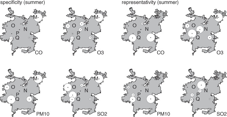
Fig. 4

Specificity (left) and representativity (right) for the univariate case for CO, O3, PM10, and SO2 for summer for seven stations during 1997–2008. The larger the circle, the larger the index.
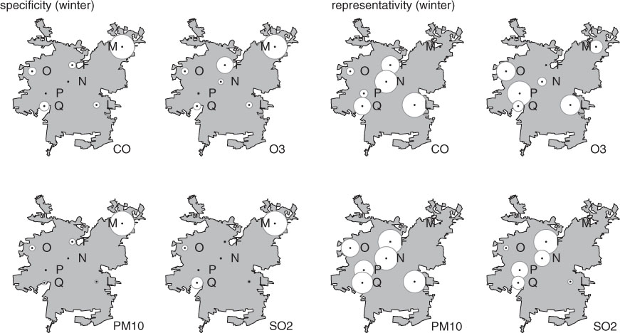
Fig. 5

Specificity (left) and representativity (right) for the univariate case for CO, O3, PM10 and SO2 for winter for seven stations during 1997–2008. The larger the circle the larger the index.
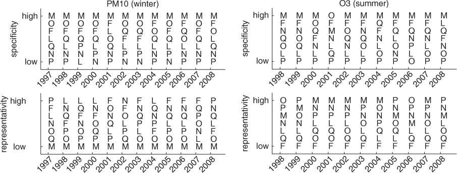
Fig. 6

Evolution of ‘specificity’ (upper panels) and ‘representativity’ (lower panels) indexes for PM10 in winter and O3 in summer respectively. See text for details.
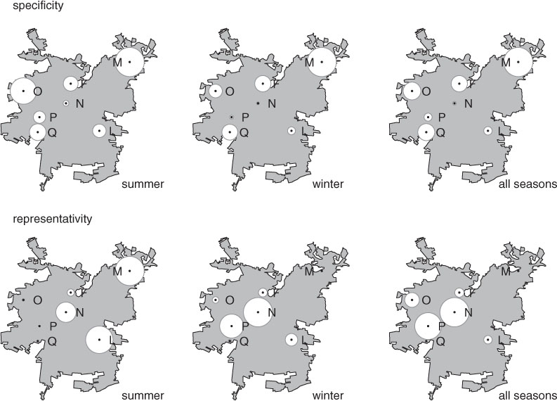
Fig. 7

Multivariate specificity (top) and representativity (bottom) indexes for simultaneously CO, O3, PM10 and SO2 for hourly data for the period 1997–2008 separately for summer, winter and all seasons.
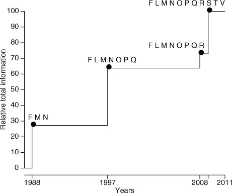
Fig. 8

Evolution of total information content of the air quality monitoring network in Santiago since the late 1980s relative to the current situation, considering PM2.5.
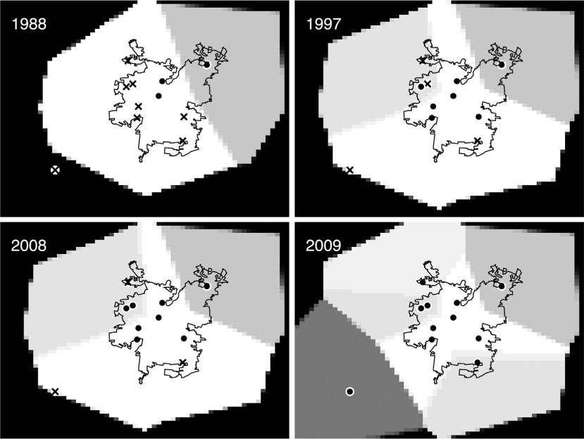
Fig. 9

Simulated interpolation of the measurements at some sites (×) from the available network (•) using Barnes interpolation (here for some typical log concentrations of PM10 in greyscale, lighter=higher). To localise, we put 12 phantom zero measurement stations around the boundary. This allows to better estimate the a priori mean μbi and covariances B i for the evolution of network total information taking into account the spatial distribution.
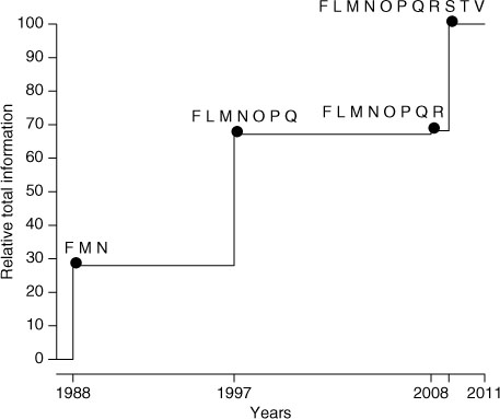
Fig. 10

Evolution of total information content of the air quality monitoring network in Santiago since the late 1980s relative to the current situation, considering PM2.5 using Barnes interpolation a priori information.
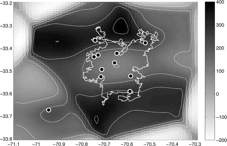
Fig. 11

Information gain map. At each point, the difference in information gain obtained by comparison of the total information gain of the original network and the total information gain obtained for a new network after adding a new station at this point with Barnes's interpolated values is indicated.
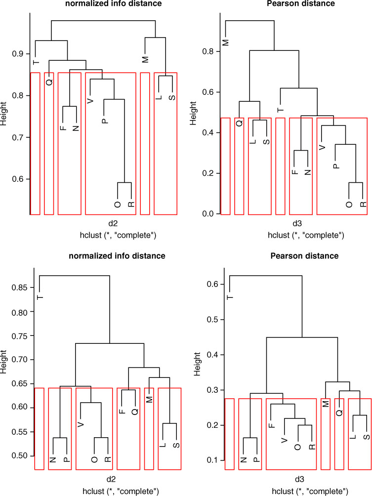
Fig. 12

Hierarchical clustering following the (not normal) normalised information distance (left column) defined in (8) compared with the Pearson correlation function (right column) for PM2.5 (top line) and O3 (bottom line).

Language: English
Page range: 19822 - 19822
Submitted on: Oct 3, 2012
Accepted on: Aug 20, 2013
Published on: Jan 1, 2013
Published by: Stockholm University Press
In partnership with: Paradigm Publishing Services

© 2013 Axel Osses, Laura Gallardo, Tania Faundez, published by Stockholm University Press
This work is licensed under the Creative Commons Attribution 4.0 License.