
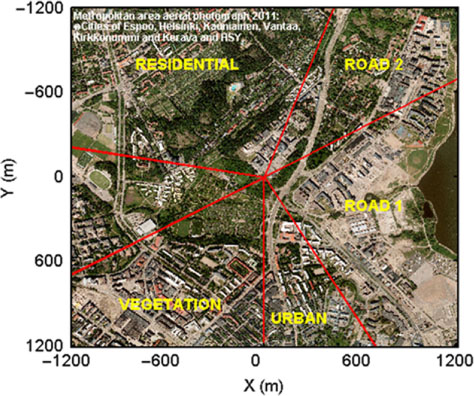
Fig. 1
Aerial photograph of the measurement site and the six sectors identified based on differences in cluster occurrences. Please note that the six sectors differ from the three areas [road (40–180°), vegetation (180–320°) and built (320–40°)] in which can be divided the surroundings of the station based on different surface cover.
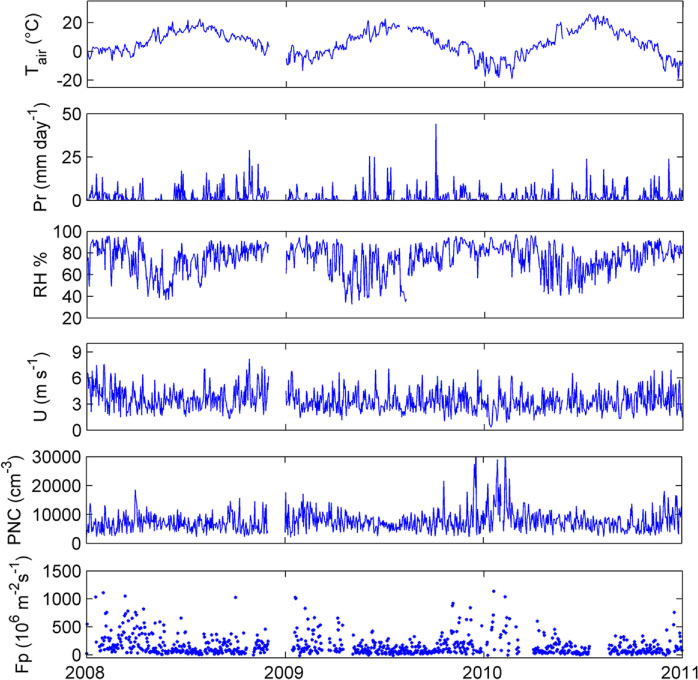
Fig. 2
Time series of daily average air temperature (T air) , precipitation (Pr, mm day−1), relative humidity (RH), wind speed (U), total particle number concentration (PNC), and vertical particle flux (F p).
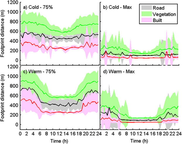
Fig. 3
The median diurnal behaviour of (a) the 75% and (b) maximum flux footprint in the road, vegetation and built sectors during the cold, and (c) and (d) the warm period. Shaded areas show the quartile deviations.
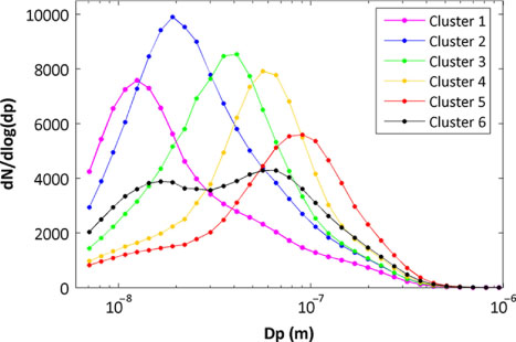
Fig. 4
The median particle number size distributions (7–950 nm) of the six identified clusters.
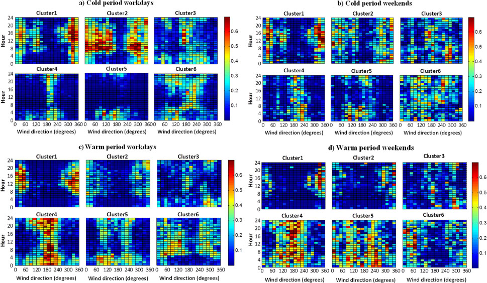
Fig. 5(a–d).
Daily occurrence of the six clusters according to the prevailing wind direction separately for cold and warm periods, and workdays and weekends. Colours represent the cluster occurrence for each hour and wind direction. Within each single period, the cross section sum of each cell having the same position in the six separate clusters is normalised to one.
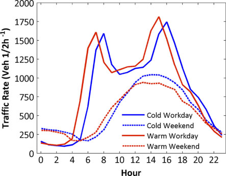
Fig. 6
Diurnal variation of traffic rate (unit) during workdays and weekends separately for the cold (October–March) and the warm period (April–September) in 2008–2010. The x-axis shows the time UTC +2 hours.
Table 1. The median PNC in size range 7–950 mm and quartile deviations for the different wind direction sectors.
Cold periodWarm periodCold periodWarm period
woWeWowewowewowe
Road 1Day (6–18)1.15±0.360.66±0.200.83±0.250.6±0.19728±327258±192423±189150±77Night (23–4)0.42±0.190.42±0.190.7±0.190.61±0.1570±4760±3733±2129±22UrbanDay (6–18)1.06±0.340.81±0.271.01±0.330.79±0.34621±270342±190301±136166±63Night (23–4)0.35±0.170.41±0.160.56±0.220.51±0.3299±58125±4749±4546±33VegetationDay (6–18)0.53±0.180.38±0.130.53±0.170.42±0.13158±7663±4287±5342±21Night (23–4)0.27±0.090.32±0.100.41±0.120.47±0.1425±1731±1614±914±11ResidentialDay (6–18)0.72±0.350.32±0.140.6±0.240.41±0.14104±5447±2564±3822±21Night (23–4)0.39±0.190.33±0.190.6±0.160.58±0.1529±1625±1317±1018±10Road 2Day (6–18)1.29±0.350.69±0.280.83±0.250.56±0.17320±136123±56217±9386±38Night (23–4)0.58±0.210.53±0.270.7±0.230.61±0.2266±2853±3128±9335±19
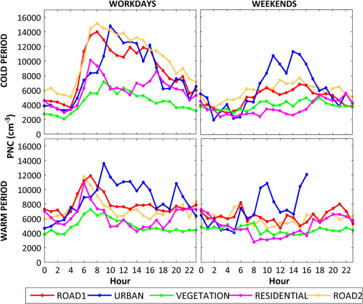
Fig. 7
Median diurnal variation of PNC in the size range 7–950 nm for the five wind direction sectors (Fig. 1) during workday and weekends separately for cold (October–March) and warm period (April–September).
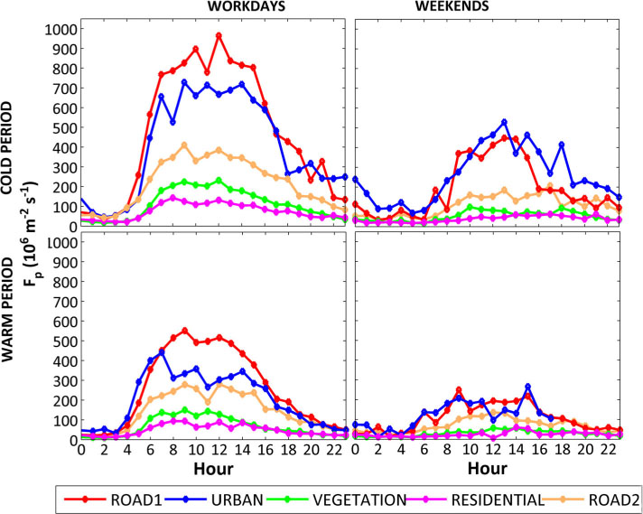
Fig. 8
Median diurnal variation of UFP vertical Flux (F p) for the five wind direction sectors (Fig. 1) during workday and weekends separately for the cold (October–March) and the warm period (April–September).
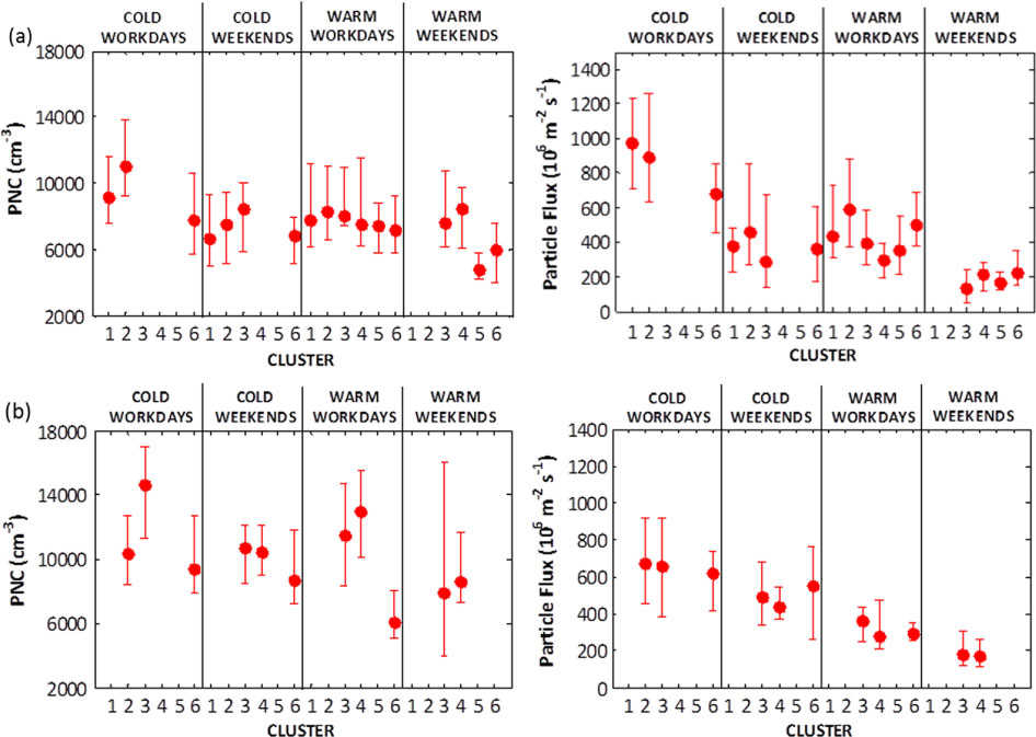
Fig. 9(a, b).
Median PNC and F p for the different cluster occurrences in Road_1 sector (a) and Urban sector (b). The median values are computed for daytime hours 10.00–15.00. See Table 2 for the amount of data used for the calculation of each data point.
Table 2. Number of data points used in the calculation of the median PNC and F p reported in Figure 9 for daytime hours 10.00–15.00 for the Road 1 and Urban sectors
ColdWarmColdWarm
Wowewowewowewowe
Cluster 1141285384060Cluster 22173290853642Cluster 321143914128587919Cluster 411511420278639Cluster 5017330111113Cluster 63421229224323372
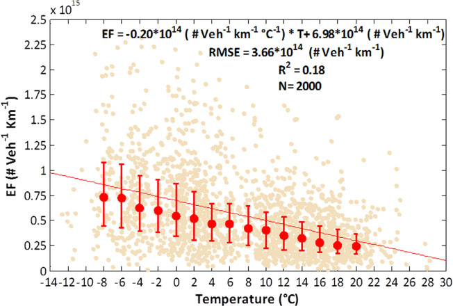
Fig. 10
The estimated 30-minute EF values (small light red dots) as a function of ambient temperature. The parameters of the linear fit of the 30-minute EFs (red line) are given in the legend. Red dots are median EFs calculated for 4° temperature bins with error bars reporting the interquartile ranges.
Table 3. Comparison of mixed vehicle fleet emission factors reported in literature studies
This studyEddy covarianceUrban road>6 nmCold 6.03±0.19Warm 3.65±0.12Järvi et al., 2009bEddy covarianceUrban road>6 nm3.0±1.1Mårtensson et al., 2006Eddy covarianceUrban road>11 nm1.4±0.1Wang et al., 2010Invers modellingUrban road10–700 nm1.87±0.03Invers modellingHighway10–700 nm2.15±0.05Ketzel et al., 2003Invers modellingUrban street canyon10–700 nm2.8±0.52004TunnelUrban road tunnel3–900 nm4.6±1.92009CFDUrban motorway10–500 nm2.1±0.2