Fig. 1.
Annual composite angular radon concentration (mBq/SCM) distributions at Cape Grim for 2001–2008, characterised by 25th, 50th, and 75th percentiles: (a) all wind directions; (b) baseline sector only. Bin width is 5 deg.
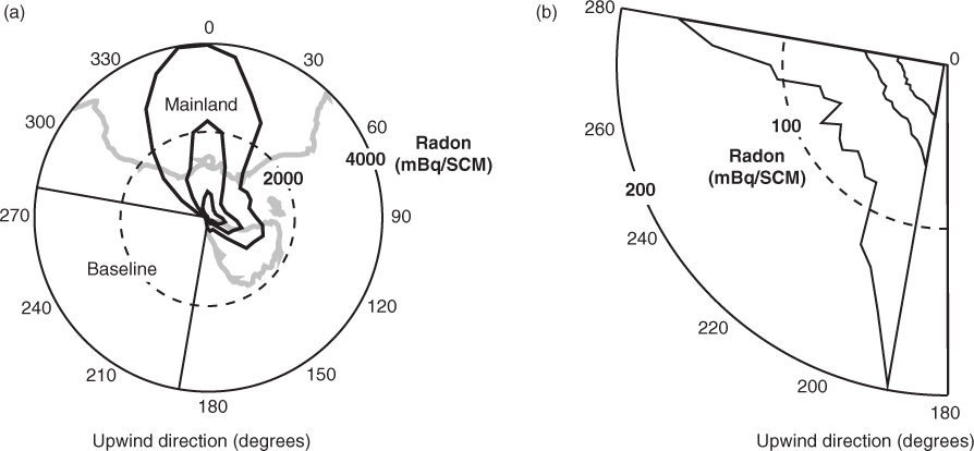
Fig. 2.
2001–2008 back trajectory density functions for all baseline observations at Cape Grim. The density is defined by (a) the time spent by trajectories in 50×50 km grid cells; (b) the mean time required by air parcels moving along trajectories to reach Cape Grim (in units of radon half-lives, T1/2=3.82 days).
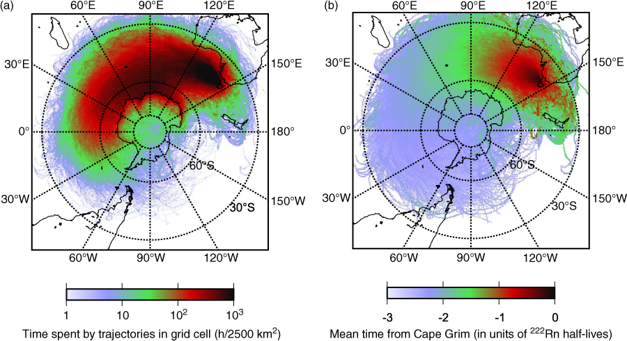
Table 1. Radon concentration (mBq/SCM) distribution at Cape Grim in 2001–2008 for baseline (local wind direction between 190° and 280°) and non-baseline conditions
Table 2. Radon concentration (mBq/SCM) distributions of baseline observations in composite year and season at Cape Grim in 2001–2008
[i] A sequence of concentration sets (from top to bottom) characterises the results of selection steps for obtaining the least perturbed radon concentration set. The sequence starts with the initial baseline observation set defined by the local wind direction only. This is followed by seven sets each of which is obtained by removing some observations from the previous set. Annual distributions of the removed observations (R1–R7) are also shown. See Section 3 for details; bold entries are depicted in Fig. 5.
Fig. 3.
Radon concentration (mBq/SCM) distribution characterised by 5th, 10th, 25th, 50th, 75th, 90th, and 95th percentiles in the baseline sector as a function of duration in the baseline sector.
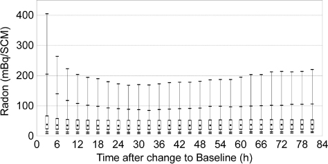
Fig. 4.
Radon concentration (mBq/SCM) distribution characterised by 5th, 10th, 25th, 50th, 75th, 90th, and 95th percentiles in the baseline sector in consecutive 3-hour period before a change to a non-baseline sector.
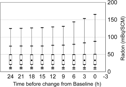
Fig. 5.
Radon concentration (mBq/SCM) distributions for the seven selection steps to extract from the initial baseline observations (Set 0 in Table 2) a set of least perturbed radon concentrations in air parcels that are in equilibrium with their oceanic radon source (Set 7 in Table 2). Each step is represented by a graph contrasting a distribution of rejected concentrations (in red) with associated distributions before and after application of the step's selection criterion shown to its left (in black) and right (in green). The number of rejected concentrations expressed as a percentage of the number of events in the initial baseline set (Set 0 in Table 2) is shown in the top right corner. All distributions are identified by their numbers shown in Table 2. Note change of the radon concentration scale between different graphs.
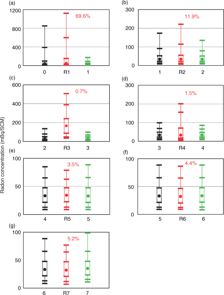
Fig. 6.
2001–2008 back trajectory density functions for least perturbed baseline observations (Set 7 in Table 2) at Cape Grim. The density is defined by the time spent by trajectories in 50×50 km grid cells.
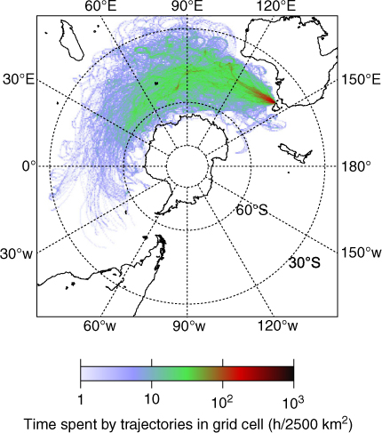
Fig. 7.
ERA-Interim mixing height (labelled model) at the closest oceanic grid point to Cape Grim compared with mini-lidar mixing height measurements at Cape Grim during 14 baseline events in 1998. An orthogonal distance regression fitting line (slope 1.03) shown on the scatter plot explains 85% of the variance.
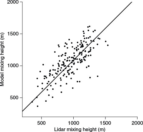
Table 3. Comparison of oceanic radon flux densities (mBq m−2 s−1) obtained in this paper (top section of the table) followed by spot measurements (accumulator and profile techniques), modelled flux, and assumed in or inferred from general circulation models
[i] aDistribution of trajectory averaged wind speeds weighted by radon decay.
[ii] bNine samples from the Southern Atlantic – the study reports 100 measurements.
[iii] cGlobal model, results shown in the table refer to the Southern Ocean only.
Fig. 8.
Oceanic radon flux density (mBq m−2 s−1) as a function of: (a) radon weighted trajectory mean wind speed (0.6 m s−1 bins), and (b) significant wave height (0.15 m bins). Whiskers show the quartile range of the radon flux density with crosses indicating the bin median and dots the bin mean. Solid lines represent a quadratic fit a*x2+c. Coefficients (variance) of the fit are for (a) a=0.000580 (1.0293*10−8), c=0.0682 (0.000721), and for (b) a=0.017 (2.798*10−6), c=0.00679 (0.000534).
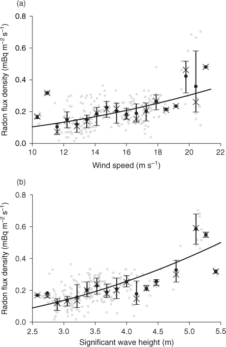
Fig. 9.
Oceanic radon flux density (mBq m−2 s−1) as a function of latitude (1° bins) for (a) summer and (b) non-summer months. Whiskers show the quartile range of the radon flux density with crosses indicating the bin median and dots the bin mean. Solid lines represent a linear fit. Coefficients of the fit are: (a) slope= −0.00667, intercept=0.135; correlation coefficient=−0.176, significance level=99.9%, and (b) slope= 0.00111, intercept= 0.314, correlation coefficient=0.034, significance level=55.3%.
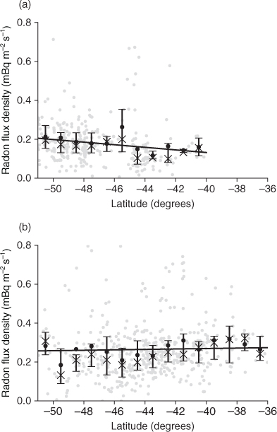
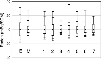
Fig. 10.
Comparison of radon concentration (mBq/SCM; relative to the median) distributions for the least perturbed set in 2002–2003 obtained from experiment (E) and averaged model (M); the contributing models’ distributions are also shown (1=AM2.GFDL; 2=AM2t.GFDL; 3=CCAM.CSIRO; 4=CCSR_NIES1.FRCGC; 5=CCSR_NIES2.FRCGC; 6=PCTM.CSU; 7=TM3_vfg.BGC). For details regarding the models see Law et al., 2008, 2010.