
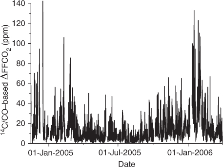
Fig. 1
Hourly 14C-calibrated CO-based fossil fuel CO2 offsets in Heidelberg relative to Jungfraujoch (cf. Section 2.1.).
Table 1. Distribution parameters in the IER2005 emission model

Fig. 2
Top: Map of the spatial distribution of FFCO2 fluxes in the year 2005. Bottom: Annual mean emission of CO2 in the immediate vicinity of the Heidelberg measurement site. The highly populated Heidelberg-Mannheim region is clearly visible as well as the large industrial area of Mannheim-Ludwigshafen. The coal-fired power plant in Mannheim approximately 20 km to the north-west of Heidelberg is also clearly distinguishable as the strongest single emitter in the region.
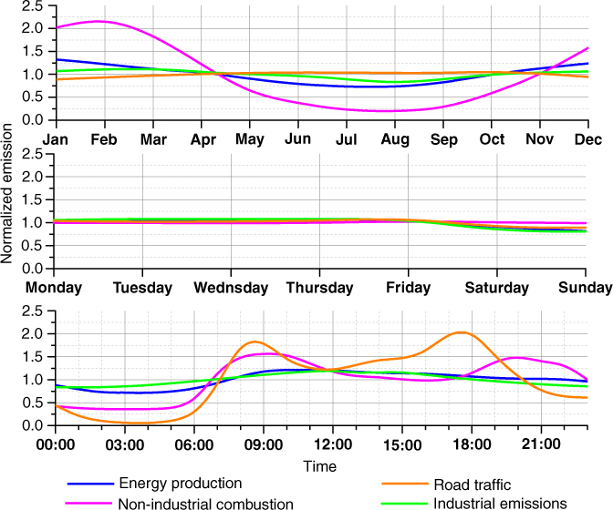
Fig. 3
Example of the temporal disaggregation of FFCO2 emissions within the IER2005 emission model for energy production (blue), non-industrial combustion (magenta), road traffic emissions (orange) and industrial emissions (green). Emission factors for monthly (upper panel), day-to-day (middle panel) and hourly (lower panel) variations of FFCO2 fluxes are shown.
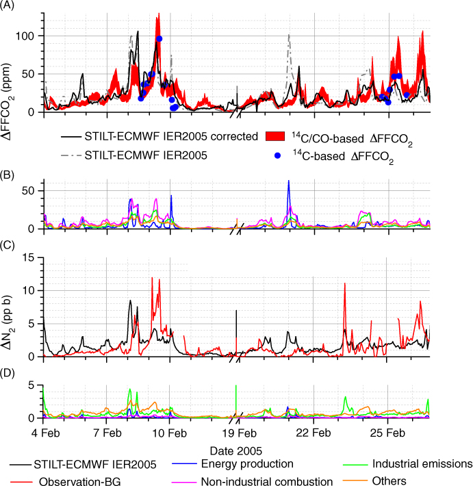
Fig. 4
Two example episodes in 2005 of observational data and modelling results derived using STILT-ECMWF and the IER 2005 emission model. (A) 14C/CO-based ΔFFCO2 measurements, including the 1-sigma uncertainty range (red band), solely 14C-based ΔFFCO2 estimate from grab samples (blue dots), and the original modelling results (grey, dotted) as well as the 222Rn-corrected model (black line). (B) Sectors contributing to the total ΔFFCO2 in the model, namely energy production (blue), non-industrial combustion (magenta), industrial emissions (green) and others in orange. (C) Modelled excess of N2O in Heidelberg (black) and the local offset of N2O derived from the observation. (D) Sectors contributing to the overall ΔN2O in the model, energy production (blue), non-industrial combustion (magenta), industrial emissions (green) and others (orange), the latter including the strongly contributing sectors for N2O: waste and agriculture.

Fig. 5
Mean diurnal cycle of ΔFFCO2 in Heidelberg pooled for A: winter (JFM) and B: summer (JJA). The 14C/CO-based regional ΔFFCO2 is given in black with its 1-sigma uncertainty range in grey. The 14C-based ΔFFCO2 from the grab samples is pooled according to the time of day and given in solid blue and the 1-sigma uncertainty range (dotted blue). The STILT-ECMWF results using the IER2005 emission model input are given in red, both the original data (dashed lines) and the 222Rn-corrected data (solid lines).
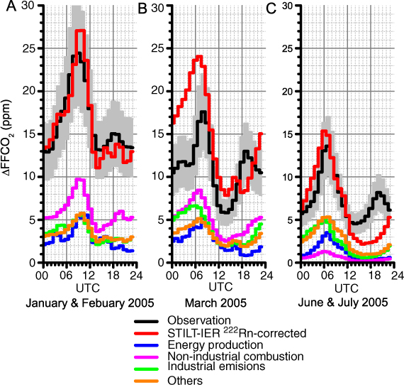
Fig. 6
Mean diurnal cycle of the local FFCO2 offset for different months in 2005, A: January and February, B: March, C: June and July. The 14C/CO-based ΔFFCO2 estimates (black, with 1σ uncertainties in grey) are compared to the radon-corrected STILT-IER2005 result (red) and the individual contributions to the modelling results (other colours).