
Table 1. Longitude and latitude of source regions shown in Fig. 1 and corresponding CO fossil fuel-biofuel/biomass burning emissions (Tg(CO)/yr) on seasonal basis in GEOS-CHEM as considered in this study
70°E–177.5°E64.8/10.764.8/39.563.3/10.264.1/2.64. Africa36°S–32°N17.5°W–70°E14.6/68.315.0/14.215.0/75.814.8/52.25. South America56°S–24°N122.5°W–32.5°W14.6/20.115.0/32.115.0/51.414.8/77.56. Oceania52°S–8°N70°E–177.5°E5.7/7.15.8/8.95.8/15.45.8/18.1Total156.4/106.4157.3/95.8154.3/158.5155.4/154.2
Table 2. CO tagged tracers considered in GEOS-CHEM according to emission sources, geographical regions and chemical production
Table 3. The main characteristics of the seasonal circulation patterns at SLP
Table 4. Contribution (%) of the CO sources to the European CO concentrations at surface, 500 hPa and 200 hPa in winter and summer of 2001
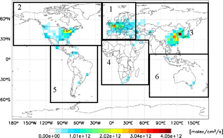
Fig. 1
Global CO anthropogenic surface emissions (in molec/cm2/s). Black boxes depict the geographical regions considered in GEOS-CHEM tagged CO analysis; 1: Europe, 2: North America, 3: Asia, 4: Africa, 5: South America, 6: Oceania.
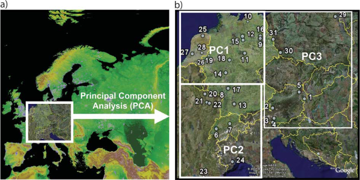
Fig. 2
a) European domain (http://www.ngdc.noaa.gov/mgg/topo/globegal.html#continents) where the 31 rural background stations are located. b) PC1, PC2 and PC3 station regions in Europe.
Table 5. Annual contribution (%) of COFFEU, COFFNA, COFFAS, COFFRW and LRT (sum of COFFNA, COFFAS and COFFRW) to CO budget at the three station regions (PCs) in 2001
(ppbv) MES
(ppbv) MB
(ppbv)ME
(ppbv)R2
COFFEU
% COFFNA
% COFFAS
% COFFRW
% LRT
%PC1217.8221.9−4.132.90.8360.17.49.00.917.3PC2208.4236.4−28.049.10.5754.78.09.71.218.9PC3265.7255.310.435.40.6855.77.69.81.218.6
[i] Statistical parameters of the observed (O) and the estimated (ES) by the nested-grid simulation of GEOS-CHEM mean monthly CO concentrations in Europe are also presented. Statistical parameters equations can be found in Appendix S5.
{ label needed for table-wrap[@id='UT0006'] }
Table 6. Percentage contribution (%) of COFFNA, COFFAS and their sum (COFFLRT) in winter at each PC sub-region in relation to the frequency of occurrence (FO) of the circulation patterns in percentage (%)
CTFOCOFFNACOFFASCOFFLRTCOFFNACOFFASCOFFLRTCOFFNACOFFASCOFFLRTW_CT1+22.25.27.112.36.07.513.56.19.615.7W_CT2+8.97.510.017.56.07.713.68.210.418.5W_CT3+0.00.00.00.00.00.00.00.00.00.0W_CT4+2.210.915.626.57.09.816.811.416.728.1W_CT5+6.73.96.210.25.88.013.86.19.115.2W_CT6+5.67.110.217.45.57.312.87.19.616.7W_CT7+12.24.86.711.45.97.913.86.69.315.9W_CT1−5.610.613.023.58.110.518.59.712.822.5W_CT2−8.910.912.623.512.814.927.78.09.817.8W_CT3−2.27.111.919.06.311.718.06.412.518.9W_CT4−7.89.913.022.910.813.824.510.614.224.8W_CT5−5.611.317.328.68.912.521.411.618.129.6W_CT6−11.19.611.521.110.011.821.88.39.818.1W_CT7−1.14.66.711.38.713.221.96.38.614.9
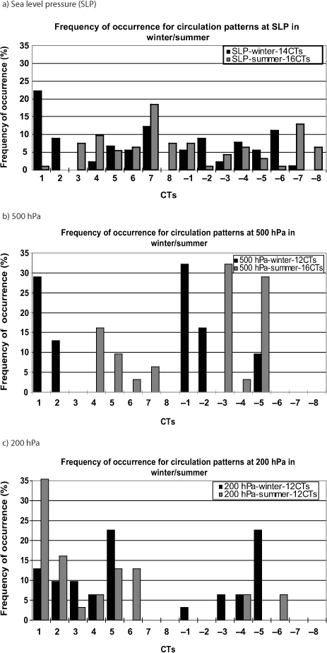
Fig. 3
Frequency of occurrence of CTs in winter and summer of 2001 at a) SLP, b) 500 hPa, c) 200 hPa.
Table 7. Percentage contribution (%) of COFFNA, COFFAS and their sum (COFFLRT) in spring at each PC sub-region in relation to the frequency of occurrence (FO) of the circulation patterns in percentage (%)
CTFOCOFFNACOFFASCOFFLRTCOFFNACOFFASCOFFLRTCOFFNACOFFASCOFFLRTSP_CT1+0.00.00.00.00.00.00.00.00.00.0SP_CT2+0.00.00.00.00.00.00.00.00.00.0SP_CT3+12.09.711.621.37.59.817.38.511.319.8SP_CT4+15.28.613.121.78.512.320.99.714.123.9SP_CT5+2.27.911.219.19.512.522.08.311.419.7SP_CT6+2.29.615.625.111.919.231.110.014.724.8SP_CT7+3.311.513.224.713.515.428.99.512.221.7SP_CT8+0.00.00.00.00.00.00.00.00.00.0SP_CT1−6.59.713.423.011.716.528.39.612.722.3SP_CT2−7.611.416.427.812.717.330.010.614.224.8SP_CT3−15.26.510.016.510.514.024.57.812.220.0SP_CT4−6.510.012.922.913.016.829.89.913.923.8SP_CT5−8.78.613.121.67.210.417.69.013.722.7SP_CT6−12.06.610.416.910.413.924.29.314.423.7SP_CT7−1.18.314.823.110.015.625.69.815.625.4SP_CT8−8.79.314.724.010.416.326.79.114.323.4
Table 8. Percentage contribution (%) of COFFNA, COFFAS and their sum (COFFLRT) in summer at each PC sub-region in relation to the frequency of occurrence (FO) of the circulation patterns in percentage (%)
CTFOCOFFNACOFFASCOFFLRTCOFFNACOFFASCOFFLRTCOFFNACOFFASCOFFLRTSU_CT1+1.14.04.48.43.64.58.14.74.99.6SU_CT2+0.00.00.00.00.00.00.00.00.00.0SU_CT3+7.69.212.922.18.311.219.68.011.119.2SU_CT4+9.87.89.317.08.911.019.97.49.917.3SU_CT5+5.46.26.112.36.16.312.46.46.412.8SU_CT6+6.56.46.813.26.87.514.35.47.212.6SU_CT7+18.56.16.112.25.96.312.16.36.813.1SU_CT8+7.64.15.39.54.45.610.05.06.111.1SU_CT1−7.68.79.318.07.39.416.78.49.818.2SU_CT2−1.14.45.39.710.38.719.17.57.114.6SU_CT3−4.36.47.513.98.18.816.86.67.013.6SU_CT4−6.56.65.712.34.95.910.85.56.211.8SU_CT5−3.34.85.710.55.06.311.45.87.413.2SU_CT6−1.15.57.312.84.76.210.96.510.216.7SU_CT7−13.05.88.914.75.47.212.56.59.616.0SU_CT8−6.510.410.621.010.410.220.67.48.515.9
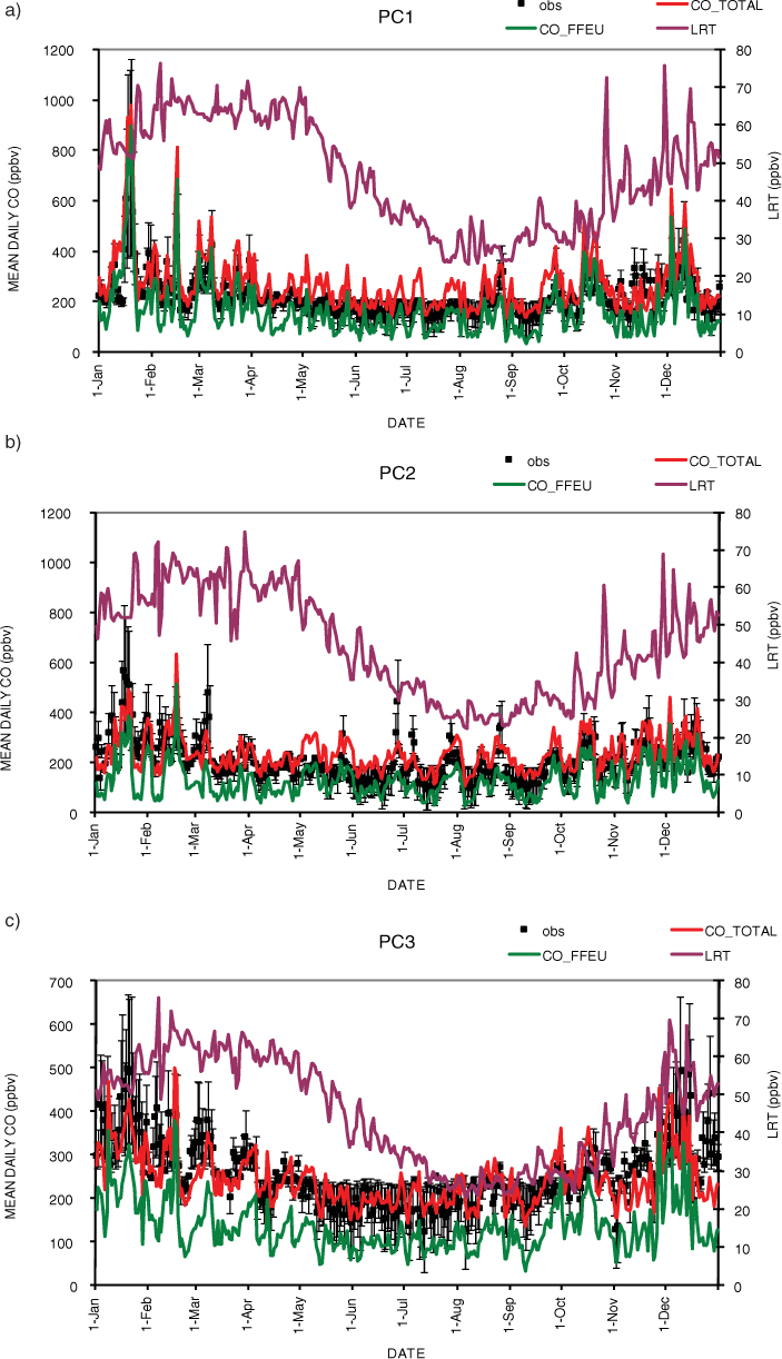
Fig. 4
Time series of the mean daily concentrations of CO measurements (black squares) and modelled concentrations of COtotal (red line) and COFFEU (green line) in the left axis and LRT (sum of COFFNA, COFFAS and COFFRW, purple line) concentrations in the right axis in 2001 at a) PC1, b) PC2, c) PC3.
{ label needed for table-wrap[@id='UT0009'] }
Table 9. Percentage contribution (%) of COFFNA, COFFAS and their sum (COFFLRT) in autumn at each PC sub-region in relation to the frequency of occurrence (FO) of the circulation patterns in percentage (%)
CTFOCOFFNACOFFASCOFFLRTCOFFNACOFFASCOFFLRTCOFFNACOFFASCOFFLRTA_CT1+0.00.00.00.00.00.00.00.00.00.0A_CT2+0.00.00.00.00.00.00.00.00.00.0A_CT3+19.89.210.419.66.97.714.69.09.718.6A_CT4+7.74.54.89.35.45.210.54.95.410.3A_CT5+7.78.35.513.810.98.018.88.26.414.6A_CT6+0.00.00.00.00.00.00.00.00.00.0A_CT7+11.09.86.716.59.88.017.87.76.814.5A_CT8+5.55.34.710.04.94.79.64.44.18.5A_CT1−8.810.98.919.98.07.315.39.48.618.0A_CT2−1.17.99.116.97.28.315.57.18.916.0A_CT3−5.54.44.38.75.24.910.15.14.69.7A_CT4−15.48.26.815.07.57.014.57.37.014.2A_CT5−0.00.00.00.00.00.00.00.00.00.0A_CT6−3.33.53.26.66.56.312.85.14.79.8A_CT7−4.45.44.810.25.35.610.85.55.611.1A_CT8−11.010.57.718.29.17.716.88.47.215.6