
Table 1. Major model characteristics
Fig. 1.
Top row: Observed annual climatology of dissolved inorganic carbon (DIC; mmol/m3), alkalinity (Alk; mmol/m3) – both taken from Key et al. (2004), and PO4 (mmol/m3) – taken from Garcia et al. (2010). Below: The difference between the simulated concentrations and the observations. DIC and Alk, originally µmol/kg, were converted using the annual salinity and SST fields of Garcia et al. (2010).

Fig. 2.
a) Standardised winter (DJF) NAO indices for the 20CR dataset (years 1911–2010; Compo et al. 2011) and all six models. b) Autocorrelation r of the winter NAO index for 20CR (red) and the model range (grey). c) The corresponding EOF 1 patterns of winter sea level pressure in the North Atlantic region (30: 80°N, 100°W: 40°E).
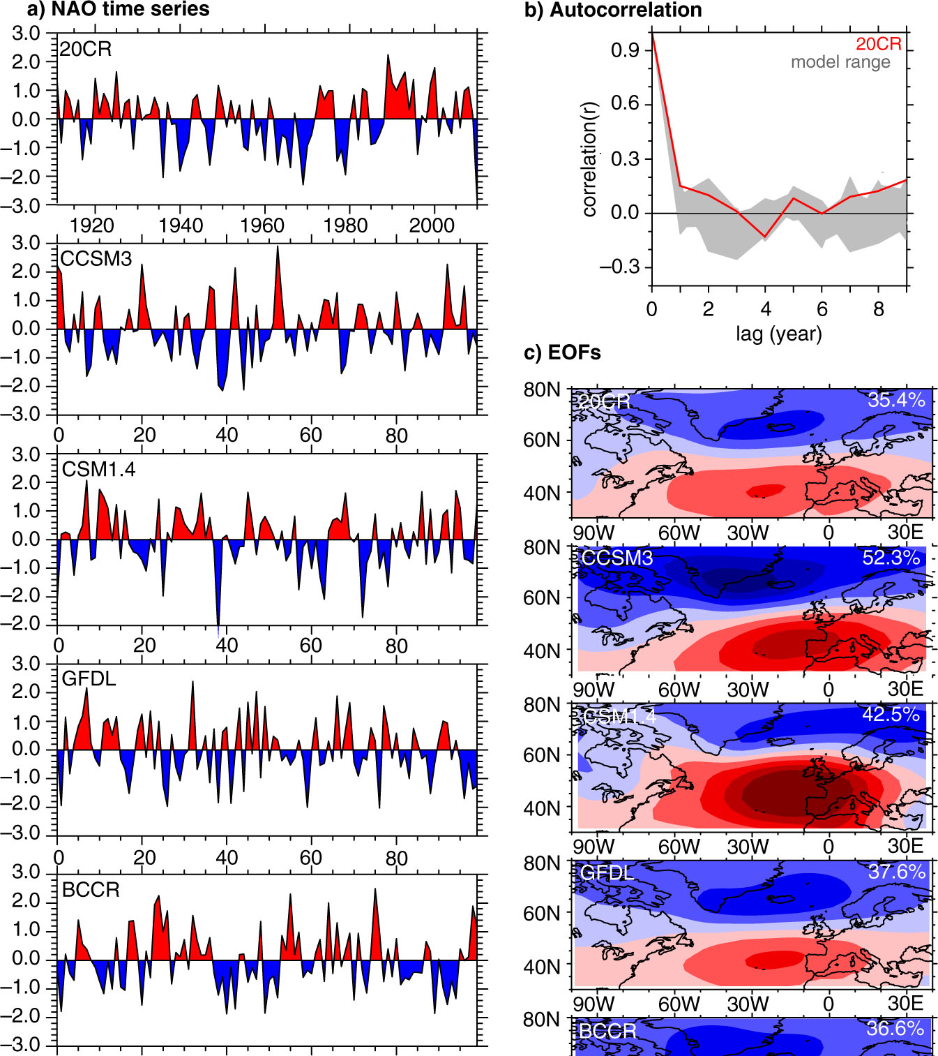
Fig. 3.
CCSM3: Correlation r with NAO index (left) and composite mean patterns for prominent NAO (NAO>|σ|; right) of wind stress (dyne/cm2), mixed-layer depth (MLD; m), barotropic stream function (BSF; Sv), upwelling (mm/s), sea-surface temperature (SST;°C) and surface salinity (SSS; g/kg). Calculations were done for the winter season and on surface level (upwelling: 75 m depth), the composites are given as anomalies and checked areas indicate statistical significance (t test, 5% level).

Fig. 4.
Model comparison: Composite mean winter patterns for prominent NAO (NAO>|σ|) of mixed-layer depth (MLD; m) and upwelling (mm/s). Upwelling is calculated at a depth of 75 m, the composites are given as anomalies and checked areas indicate statistical significance (t test, 5% level). For BCCR, an isopycnic model, upwelling is not available.

Fig. 5.
CCSM3: Correlation r with NAO index (left) and composite mean patterns for prominent NAO (NAO>|σ|; right) of dissolved inorganic carbon (DIC; mmol/m3), alkalinity (Alk; meq/m3), PO4 (mmol/m3), export production (POC; mmol POC/m3 cm/sec), total pH (Lueker et al., 2000) and the saturation state of aragonite (OmegaA). Calculations were done for the winter season and on surface level (POC: 75 m depth), the composites are given as anomalies and checked areas indicate statistical significance (t test, 5% level).
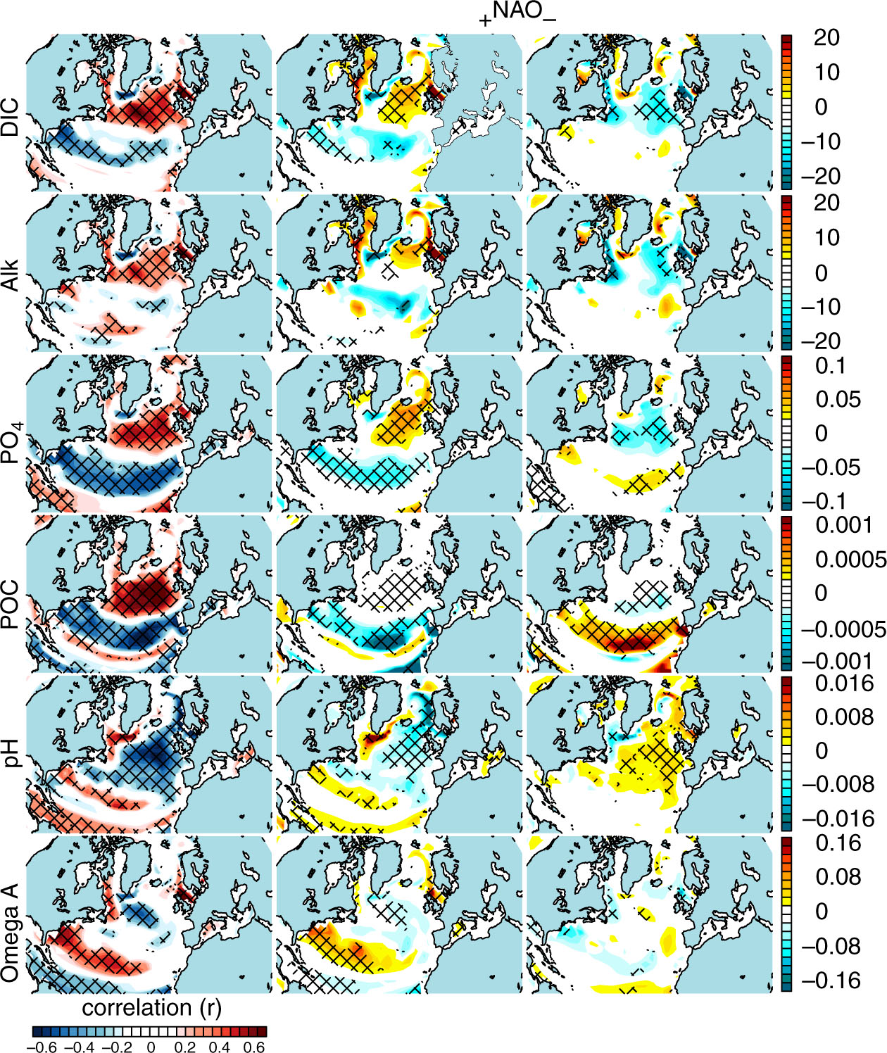
Fig. 6.
Model comparison: Composite mean winter patterns for prominent NAO (NAO>|σ|) of dissolved inorganic carbon (DIC; mmol/m3) and PO4 (mmol/m3). Calculations were done on surface level, the composites are given as anomalies and checked areas indicate statistical significance (t test, 5% level).
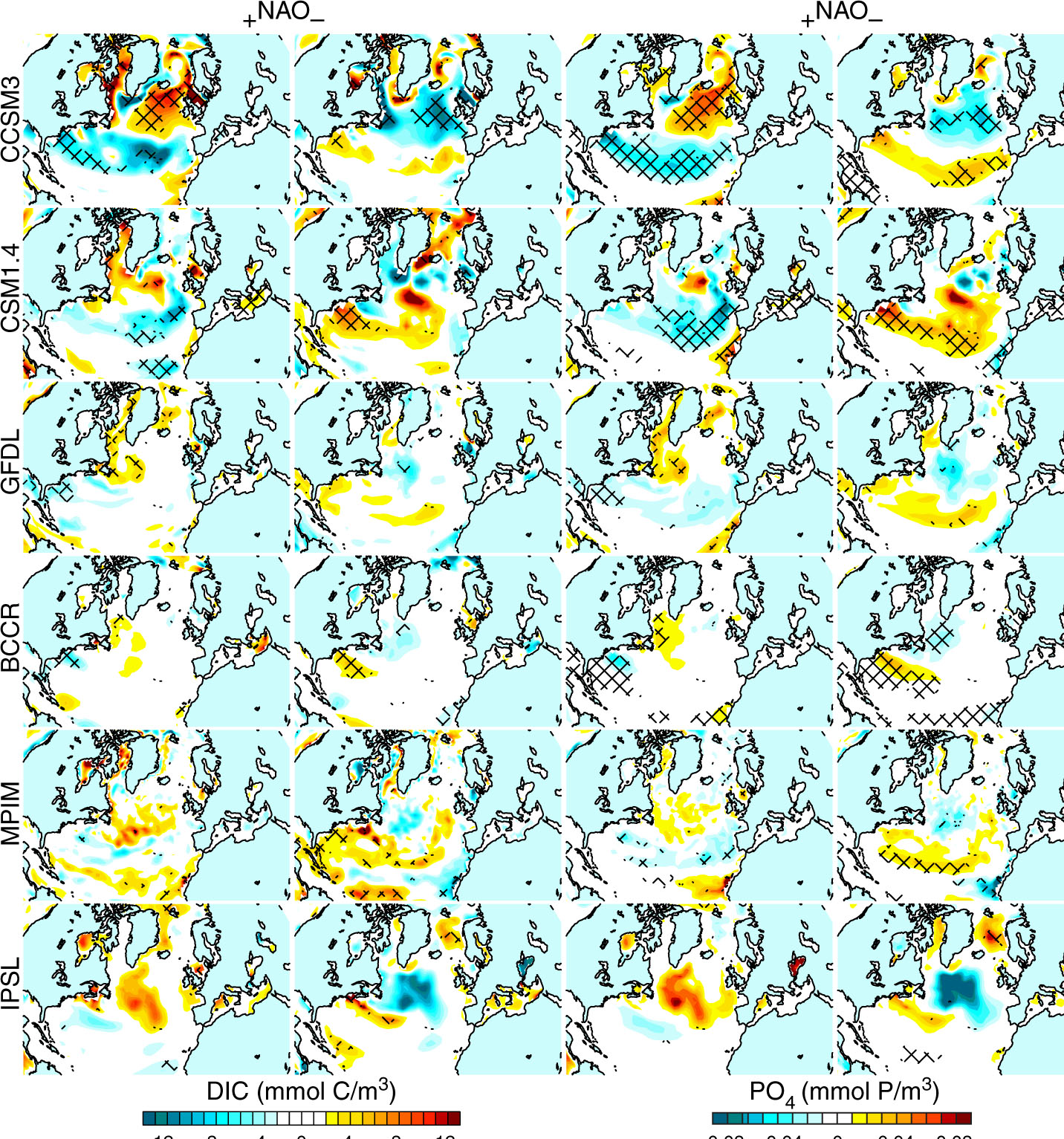
Fig. 7.
Model comparison: Composite mean winter patterns for prominent NAO (NAO >|σ|) of the gradient of pCO2 between atmosphere and ocean (ΔpCO2) and air–sea CO2 flux (mmol/m3 cm/s). Calculations were done on surface level, the composites are given as anomalies and checked areas indicate statistical significance (t test, 5% level). The unit of ΔpCO2 is ppmv (CCSM3, CSM1.4, MPIM) and µatm (GFDL, BCCR, IPSL), respectively. For the integrated annual air–sea CO2 flux (mol m−2 yr−1), multiply by 315.36.
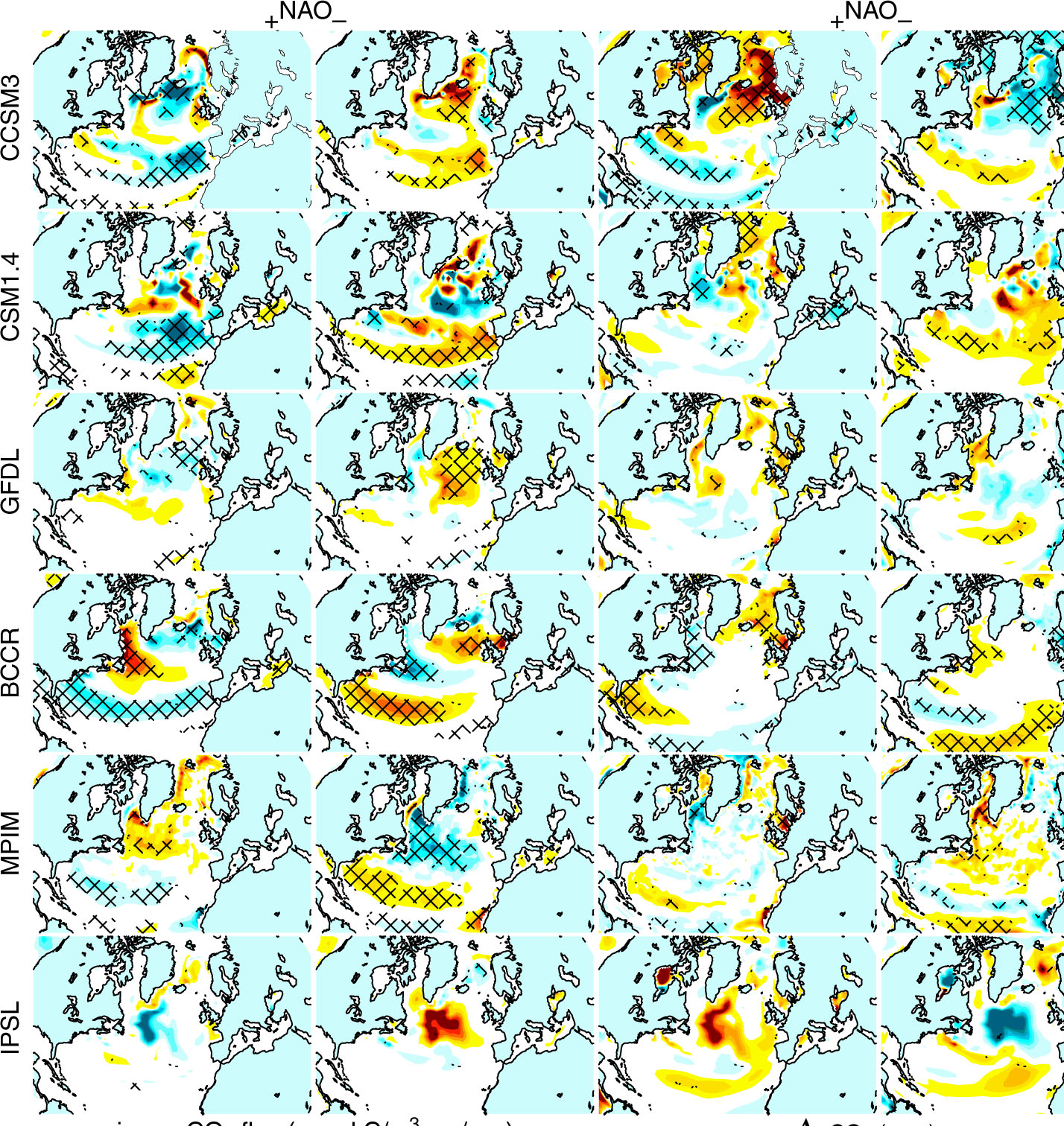
Fig. 8.
CCSM3: Anomalies of wind stress (dyne/cm2), barotropic stream function (BSF; Sv), mixed-layer depth (MLD; m), sea-surface temperature (SST; °C) and dissolved inorganic carbon (DIC; mmol/m3) during five consecutive winter seasons with positive NAO.
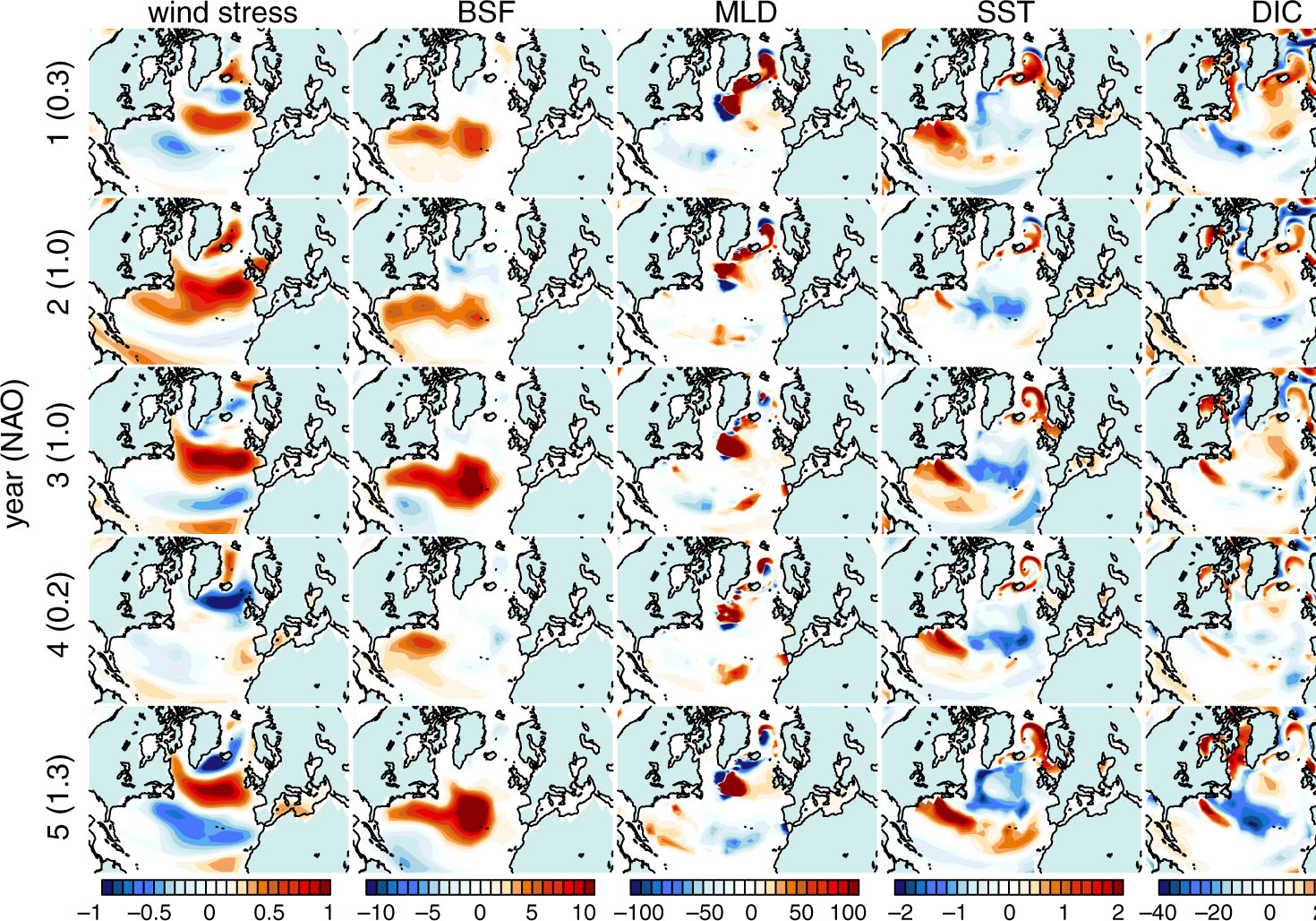
Fig. 9.
CCSM3: Time series of winter NAO index (shaded), surface dissolved inorganic carbon (DIC; mmol/m3) (blue) and mixed-layer depth (MLD; m) (red). DIC and MLD are averaged over areas in the subpolar (40: 60°N, −50: −20°E) and subtropical (29: 34°N, −67: −61°E) gyres and given as anomalies. The NAO index is standardised, arising from an EOF analysis of sea level pressure in the North Atlantic (30: 80°N, −100: 40°E).
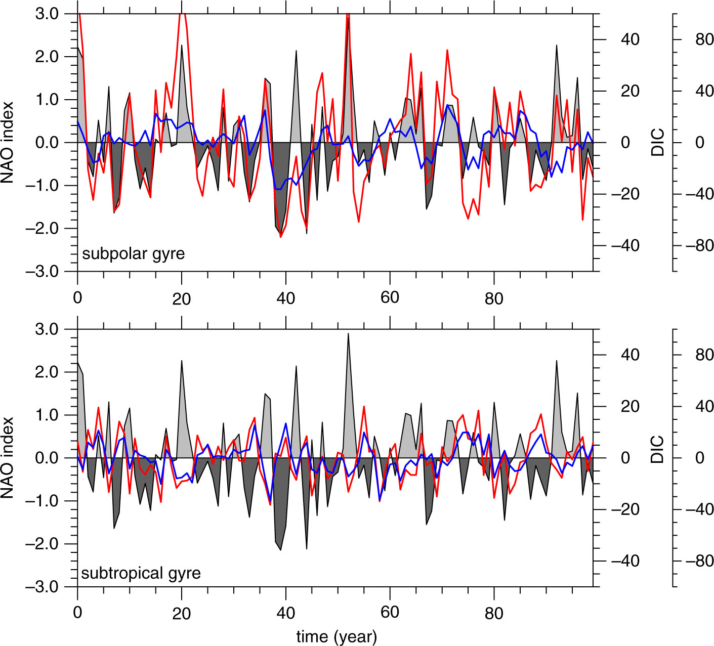
Table 2. Correlation r between monthly and seasonal (DJF) time series of NAO index and the surface variables dissolved inorganic carbon (DIC; µmol/kg), PO4 (µmol/kg) and SST (°C) for four observational datasets
[i] One dataset is an extract from BATS (Bates, 2007), located in the western subtropics (32°50′N, 64°10′W). The subpolar gyre is represented by SURATLANT (Metzl et al., 2010), covering parts of the subpolar gyre (50 : 60°N, 40 : 20°W), and measurements done on cruises in the Irminger Sea (62 : 65°N, 30 : 20°W) and Iceland Sea (62 : 65°N, 15 : 10°W) (Olafsson, 2007a, b). The NAO is represented by the NOAA CPC monthly NAO time series (http://www.cpc.noaa.gov/data/teledoc/telecontents.shtml). The variables are correlated on two temporal scales, monthly and for the winter season. For the latter, the observations comprise the available monthly values for January, February and December.
Table 3. Correlation r between monthly and seasonal (DJF) time series of NAO index and the surface variables dissolved inorganic carbon (DIC; mmol/m3), PO4 (mmol/m3) and SST (°C) for the six models
[i] The model data is averaged over areas representing the subpolar (50: 60°N, −40: −20°E) and the subtropical gyre (29: 34°N, 67: 61°W), the NAO is defined by an EOF analysis of sea level pressure in the North Atlantic (30: 80°N, 100°W: 40°E). The variables are correlated on two temporal scales, monthly and for the winter season. For the latter, the models are represented by seasonal (DJF) means.
Fig. 10.
Response of ocean physics and biogeochemistry in the North Atlantic to NAO+ forcing. To maintain a certain clarity, the scheme is simplified. For instance, pCO2 depends not only on DIC and Alk, but also on SST and salinity.
