
Fig. 1.
Seasonal anomaly of air–sea O2 flux for (top) June and (bottom) December computed by (left) our ocean biogeochemical model and (right) from the fluxes of Garcia and Keeling (2000). Positive values correspond to outgassing.
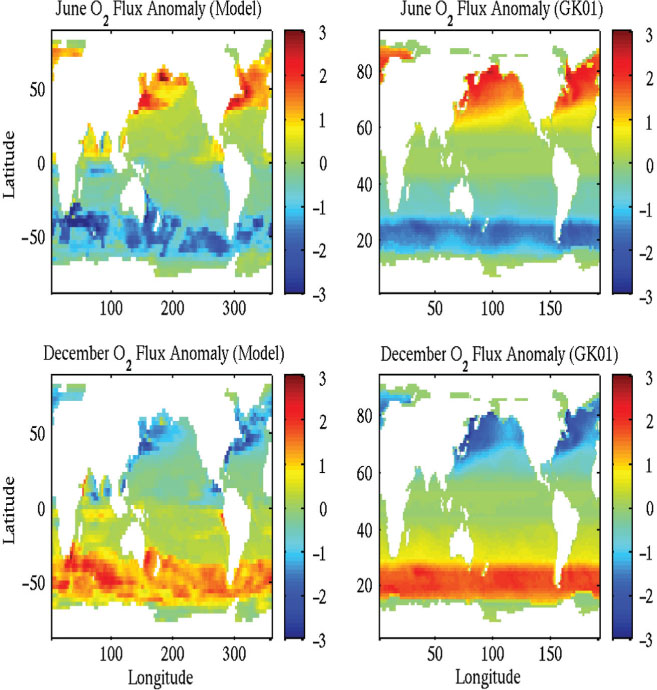
Fig. 2.
Vertical sections of [N2O] in four locations of the global ocean as computed by the ocean biogeochemical model. Values refer to annual mean and units are nM.
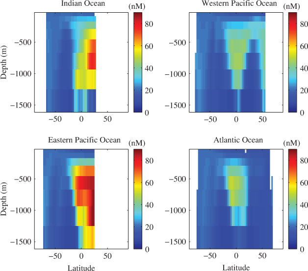
Fig. 3.
Vertical sections of observed [N2O] in four locations of the global ocean. Units are nM.
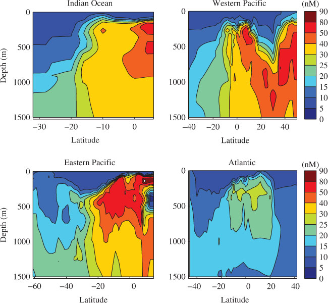
Fig. 4.
Annual mean of air–sea fluxes of total N2O computed by the ocean biogeochemical model. Units are mg N m−2yr−1.
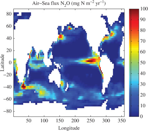
Fig. 5.
Global zonal average of the seasonal cycle of modelled quantities. Panel a compares the flux due to the production (F (Prod), green line) with the net euphotic zone production (NEZP, black line); panel b shows single components of the air–sea O2 flux; panel c shows air–sea N2O flux; and panel d shows heat flux for the latitudinal band between 10°N and 10°S as zonal average. In panels b and c, the full blue line indicates the total flux, the full red line the thermal component, the dashed magenta line the ventilation component and the full green line the production component. The first 6 months are repeated to show one and a half annual cycles. Positive values indicate both outgassing and ocean heat gain. Units are mol m−2 yr−1 for air–sea gas fluxes, and W m−2 for heat fluxes.
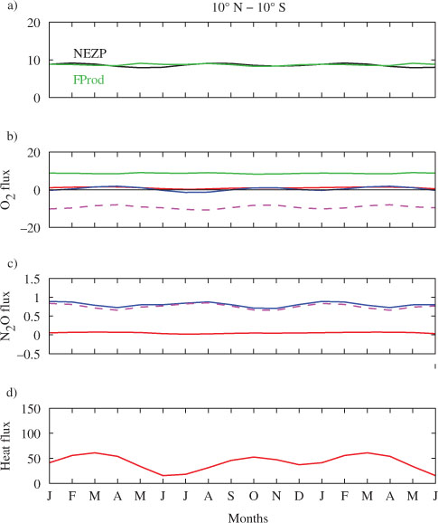
Fig. 6.
Global zonal average of the seasonal cycle of modelled quantities. Panels a and e compare the flux due to the production (F (Prod), green line) with the net euphotic zone production (NEZP, black line); panels b and f show single components of the air–sea O2 flux; panels c and g show air–sea N2O flux; and panels d and h show heat flux for the latitudinal band between 10° and 30° of each hemisphere as zonal average. In panels b, c, g and f, the full blue line indicates the total flux, the full red line the thermal component, the dashed magenta line the ventilation component and the full green line the production component. The first 6 months are repeated to show one and a half annual cycles. Positive values indicate both outgassing and ocean heat gain. Units are mol m−2 yr−1 for air–sea gas fluxes and W m−2 for heat fluxes.
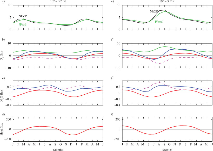
Fig. 7.
Same as previous figure but for high latitude bands (>30°) of each hemisphere.
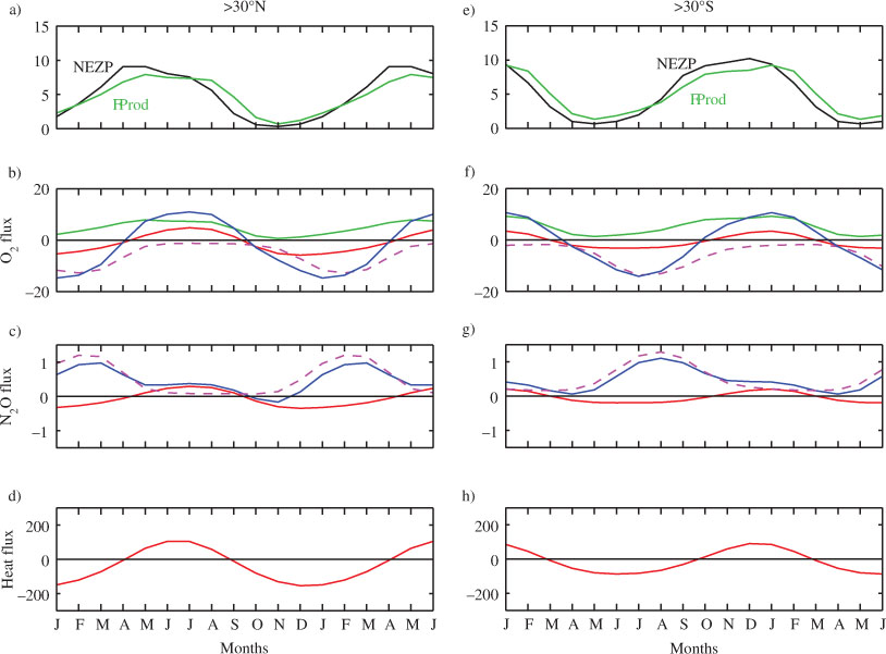
Fig. 8.
Time/latitude plot of the natural logarithm of the ratio between the ventilation and production components of the air–sea O2 fluxes for the global ocean (top left), Atlantic (top right), Pacific (bottom left) and Indian oceans (bottom right). Values are unit less and zonally averaged for each basin. Colour bar is in natural logarithmic scale.
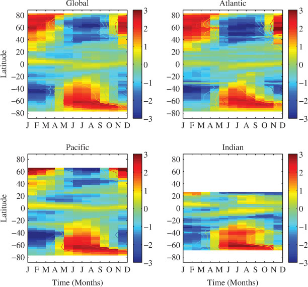
Fig. 9.
Scatter plot of components of air–sea fluxes of O2 and N2O due to ocean ventilation in different latitudinal sectors of the global ocean. Units are mol m−2 yr−1 and mmol m−2 yr−1 for O2 and N2O fluxes, respectively. The blue line represents gas–gas relationship according to each slope value calculated using a least-square fit. Positive values indicate outgassing.
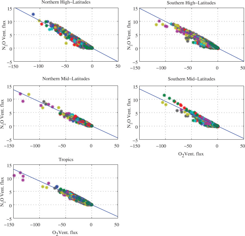
Table 1. List of ratios of ventilation fluxes of O2 and N2O for five selected latitudinal bands where a zonal average is applied
[i] We report the maximum values that correspond to the phase of ventilation between ocean surface and subsurface. Standard deviation is indicated in parenthesis and units are mmol/mol.
Fig. 10.
Zonal average of the seasonal cycle of air–sea thermal O2 flux of, from top to bottom, northern high-latitudes (>30°N); northern mid-latitudes (10–30°N); tropics (10°N–10°S); southern mid-latitudes (10–30°S); and southern high-latitudes (>30°S). The full line indicates the flux prognostically computed by the OGCM, the dotted line indicates the flux computed using the diagnostic formula of Keeling and Shertz (1992) based on ocean heat-fluxes and the dashed line indicates the air–sea flux calculated with both delaying and reduction factors according Jin et al. (2007). The first 6 months are repeated to show one and a half seasonal cycles. Positive values indicate outgassing.
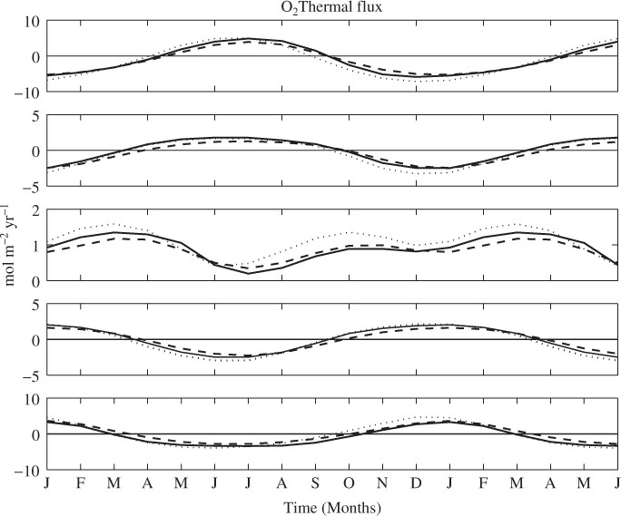
Table 2. List of ratios of flux amplitude and (in parenthesis) difference in time lag corresponding to the seasonal peak and for each latitudinal band (first column)
[i] The second column gives values of the ratio of the thermal fluxes of O2 from the OGCM over that computed according to Keeling and Shertz (1992) using the modelled net heat flux while in the third column we used the total O2 computed by the OGCM instead of the thermal flux. Calculations are based on fits to global zonally averaged fluxes over indicated latitude bands. Ratios have no units and lags are indicated in days.
Table 3. Scaling factors between air–sea gas fluxes calculated by (left) heat-flux formulas and by (right) the use of the ocean general circulation model (OGCM) used for this study
[i] Values in parenthesis indicate the correlation coefficients calculated for the OGCM output.