
Table 1. Mean concentrations of acetic end formic acids in the gaseous phase of recent polar atmosphere
[i] Concentrations are expressed in pptv. De Angelis, unpublished data: (1) mean concentrations calculated over the whole sampling period; (2) background mean concentrations – beginning of the field season; (3) and (4) mean concentrations of two successive broad peaks observed during the second part of the field season.
Fig. 1.
Acetate concentration distributions obtained along the 580 upper metres of EDC and corresponding to the Holocene (left), last glacial – interglacial transition (middle) and LGM (right) time periods. Black bars refer to the whole set of samples and grey bars refer to samples estimated to be reliable, following the sorting procedure described in Section 2.

Fig. 2.
Concentration depth profiles of acetate, formate, oxalate (left, from top to bottom, respectively), nss calcium, ammonium and nss sulphate (right, from top to bottom, respectively) along a 160-cm pit dug in summer 1997–1998 at DC site. The white dash-dotted lines on each graph delineate the range of Holocene values (Holocene mean value±SD, when corresponding to a negative value the lower line is not shown). The time scale is given by the nss sulphate peak centred at 42–52 cm deep and attributed to Pinatubo stratospheric deposits in 1992–1993. See text for concentration peaks marked A, B, C, D, E and F.
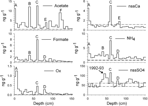
Fig. 3.
EDC (left) and EDML (right) depth profiles of nss calcium, sodium, nss sulphate, ammonium and acetate. Concentrations are expressed in ng g−1 (left axes) and deposition fluxes are expressed in ng cm−2 yr−1 (right axes). EDC: grey dots correspond to concentrations measured in samples from chemistry strips (see text), thin black lines (grey lines) correspond to mean concentrations (deposition fluxes) calculated for every chemistry strip and to concentrations (deposition fluxes) measured in samples from central lamellae and thick black lines correspond to five samples concentration running means. EDML: thin black (grey) lines indicate concentrations (deposition fluxes) and thick black lines indicate the five samples concentration running means. The climate reference along EDC is given by the deuterium profile (top) and the age scale is indicated on the graphs’ upper axes. The main climate stages recorded along EDML are indicated on the sodium graph and the age scale is indicated on the graphs’ upper axes.
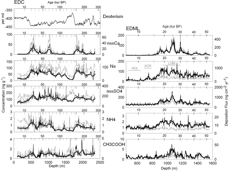
Fig. 4.
Inter-species relationships (concentrations are expressed in ng g−1). From top to bottom: ammonium as a function of nss sulphate, ammonium as a function of sodium, acetate as a function of nss sulphate, acetate as a function of sodium, acetate as a function of ammonium and acetate as a function of nss calcium. EDC (left part): grey circles and white triangles correspond to the past 30 kyr (Holocene and LGM, samples reprocessed in 2001 and 2002), white triangles cover the 24–26.5 kyr BP time period (see text) and white circles correspond to the remaining part of the last climatic cycle (30–120 kyr BP, samples reprocessed in 2003 and 2006). EDML (right part): white triangles correspond to 24–28 kyr BP (see text) and grey triangles correspond to the remaining part of the past 50 kyr.
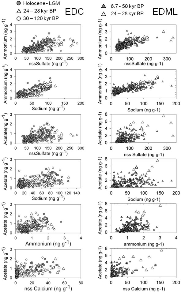
Table 2. Mean concentrations/deposition fluxes and corresponding SDs of acetate, formate, nitrate, sodium, ammonium, nss sulphate and nss calcium calculated along selected sections of EDC and EDML ice cores (see Section 3.2)
[i] Concentrations and deposition fluxes are given in ng g−1 and in ng cm−2 yr−1, respectively. LGM (1) corresponds to the part of the LGM when very high concentrations of acetate, nitrate and nss calcium are observed in EDML (see text) and LGM (2) corresponds to the remaining part of the LGM.
Fig. 5.
(a) From top to bottom: EDML depth profiles of ionic balance H+ (black line, right axis), nitrate (grey line, left axis) and nss calcium (black line, left axis); (b) EDML concentration depth profile of acetate. Ionic balance is expressed in µEq l−1. Concentrations are expressed in ng g−1.
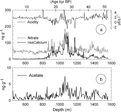
Fig. 6.
Relationships between non-sea-salt calcium and non-sea-salt sulphate deposition fluxes along EDC (top – mean deposition fluxes, when corresponding to chemistry strips) and EDML (bottom) for the past 55 kyr. White dots and white triangles correspond to the LGM (18–30 kyr BP), white triangles cover the 24–28 kyr BP time period (see text) and grey dots correspond to the remaining part of the samples. Linear regression lines and correlation coefficients corresponding to the LGM are also indicated; deposition fluxes are expressed in ng cm−2 yr−1.
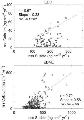
Fig. 7.
EDC (left) and EDML (right) depth profiles of formate. Concentrations are expressed in ng g−1 (left axes) and deposition fluxes are expressed in ng cm−2 yr−1 (right axes). EDC: grey dots correspond to concentrations measured in samples from chemistry strips (see text), thin black lines (grey lines) correspond to mean concentrations (deposition fluxes) calculated for every chemistry strip and to concentrations (deposition fluxes) measured in samples from central lamellae and thick black lines correspond to five samples concentration running means. EDML: thin black (grey) lines indicate concentrations (deposition fluxes) and thick black lines indicate the five samples concentration running means. The climate reference along EDC is given by the deuterium profile (top) and the age scale is indicated on the graphs’ upper axes. The main climate stages recorded along EDML are indicated on the sodium graph and the age scale is indicated on the graphs’ upper axes.
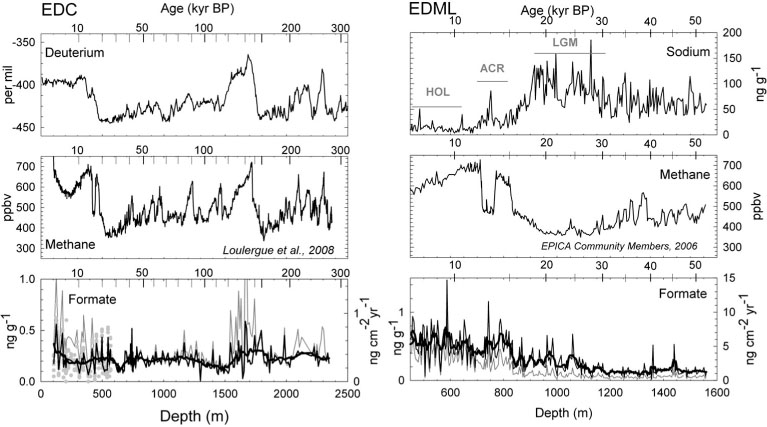
Fig. 8.
Antarctic map showing the location of sites shown in Table 3.

Table 3. Comparison of EDC and EDML Holocene mean concentrations of acetate, formate, oxalate, ammonium, nitrate and sodium with concentrations measured in firn and ice layers of other remote sites (corresponding SDs are in parentheses)
[i] Dome Summit data are from Legrand and de Angelis (1995) and Savarino and Legrand (1998). San Valentin data are from Vimeux et al. (2008). D10 data are from Legrand and de Angelis (1995) and Legrand (1985): concentration ranges correspond to the Holocene part of the core assumed to originate 300–400 km inland and the accumulation rate is deduced from present surface data measured 350–500 km from the coast along the DDU DC transect (Magand, personal communication). Other data are unpublished data from authors.