
1. Introduction
The rising atmospheric CO2 concentration and the resultant climate change may alter carbon (C) cycles of terrestrial ecosystems (IPCC, 2007), which may, in turn, amplify or dampen climate change (i.e., positive or negative C-climate feedback) (Friedlingstein et al., 2006; Luo, 2007; Heimann and Reichstein, 2008). To better understand responses of terrestrial ecosystems to climate change, it becomes essential to quantify ecosystem C uptake. The C-uptake capacity in plant and soil pools is largely determined by both C residence time and net primary productivity (NPP) changes (Luo et al., 2003). The spatial patterns of NPP changes were relatively well qualified by using ecosystem production models with remote sensing techniques in North America (Hicke et al., 2002). The former, C residence time, is the length of time that a carbon atom can stay in a reservoir from the entrance to the exit (Barrett, 2002; Luo et al., 2003). Several methods have been used to estimate the C residence time, such as C balance method via calculating ratios of C pools divided by fluxes (Vogt et al., 1996), time series decomposition experiments (Powers et al., 2009), C isotope tracing (Gaudinski et al., 2001) and inverse analysis (Barrett, 2002; Luo et al., 2003; Xu et al., 2006). However, uncertainties in estimated C residence time have not been well quantified. If the issue of uncertainty is not adequately addressed, C sink potentials cannot be fully understood and policies to mitigate climate change based on the current understanding of terrestrial C sequestration will fall short in meeting targets of the Kyoto protocol. Therefore, quantifying uncertainties of C residence times, especially at regional scales, is crucial for an improved understanding of terrestrial C uptake (Randerson et al., 1999; Barrett, 2002).
Most of the uncertainties studies have been conducted by sensitivity analysis with a local design via changing one parameter at a time while keeping the other parameters constant (Kremer, 1983; Knorr, 2000; El Maayar et al., 2002; Larocque et al., 2008) or using minimum and maximum values from the literature (Hallgren and Pitman, 2000; Zaehle et al., 2005) in ecological modelling. Although these approaches can identify uncertainty of a single parameter (Kleijnen, 1998), they neglect possible interactions between parameters and can not specify the confidence intervals for parameter distributions, which are very important in complex ecosystem models (Saltelli et al., 2000). Highly correlated parameter sets and large confidence intervals for parameter estimates would tend to indicate equifinality (i.e., the optimal parameter set is not uniquely defined) (Beven, 2006), and may increase the uncertainties in model prediction as a result of high variation in parameterisation (Schulz and Beven, 2003). In addition, non-linearity of ecosystem models may introduce considerable errors in the flux and pool estimates (Raupach et al., 2005; Zhou et al., 2008).
Only a few studies have so far assessed stochasticity and uncertainties of C residence time with inverse analysis (Wang et al., 2001; Xu et al., 2006; Larocque et al., 2008). For example, Xu et al. (2006) found that only three or four of seven parameters were well constrained by six ecological data sets collected from the Duke Free-Air CO2 Enrichment (FACE) experiment while the other parameters were unconstrained with large uncertainties. The uncertainties in estimated parameters were propagated to model projections of C sink sizes. On regional and global scales, uncertainties have usually been analysed by inversion of measured atmospheric CO2 concentration in conjunction with atmospheric transport models (Kaminski et al., 2002; Rayner et al., 2005; Prihodko et al., 2008). The atmospheric inversion can estimate regional C source/sink but cannot resolve the spatial distribution of terrestrial C sink. This is mainly due to the lack of information to enable an orthogonal decomposition of the different types of C source/sink and the uneven distribution of the measurements for atmospheric transport models (Wang et al., 2001; Wang and Barrett, 2003; Ahmadov et al., 2009; Pillai et al., 2010, 2011). Inclusion of multiple sources of information has the potential to improve parameter constraint and reduce uncertainties (Barrett, 2002; Wang and Barrett, 2003; Xu et al., 2006).
Among various inverse techniques, Bayesian inversion may be currently the most common approach to parameter estimation and uncertainties analysis (Enting, 2002; Larocque et al., 2008). It combines information from prior knowledge, model structure and data to allow the simultaneous determination of all parameters. The Markov chain-based Bayesian method can not only better account for non-linearity in the model and correlations among parameters, but also provide more robust estimates of uncertainties in parameters and model predictions by generating a probability distribution (Braswell et al., 2005; Xu et al., 2006; Prihodko et al., 2008). The Bayesian paradigm starts with prior probability distributions of parameters and then assimilates measurements into models to generate posteriori probability density functions (PDFs) of model parameters and forecasted state variables (Braswell et al., 2005; Knorr and Kattge, 2005; Xu et al., 2006). PDFs may contain information on key uncertain properties of climate change simulations (mainly CO2 concentration and temperature, Murphy et al., 2004) and ecosystem responses to elevated CO2 (Xu et al., 2006). A cumulative distribution function (CDF) has also been presented to assess the uncertainties of dangerous anthropogenic interference in model predictions of future climate change (Mastrandrea and Schneider, 2004). On regional and global scales, the Bayesian method, to our knowledge, has not been used for uncertainty analysis with multiple ecological data sets, although it has been applied to constrain parameters and for uncertainties analysis in biosphere models against atmospheric CO2 concentration data (Kaminski et al., 2002; Rayner et al., 2005; Prihodko et al., 2008).
The objectives of this study were to quantify C residence time and NPP-driven ecosystem C uptake, and their uncertainties in the conterminous USA. We first applied the Bayesian probability inversion and Markov Chain Monte Carlo (MCMC) technique to a terrestrial ecosystem regional (TECO-R) model. The 13 spatially distributed observational data sets of C pools and fluxes have been used to constrain TECO-R model for each biome (totally eight biomes) to generate posterior PDFs of 22 parameters. C residence times of ecosystem and each pool were estimated from these parameters for each of the eight biomes. Second, standard deviation (SD) and coefficient of variation (CV=SD/mean) of all estimated parameters and C residence times were calculated from posterior PDFs to represent their uncertainties. Finally, the propagation of parameter uncertainties to modelled ecosystem C uptake was assessed.
2. Materials and methods
2.1. Model description
In this study, a TECO-R model was developed by combining the Carnegie-Ames-Stanford-Approach (CASA) model (Potter et al., 1993; Field et al., 1995) with the Vegetation-And-Soil-carbon-Transfer (VAST) model (Barrett, 2002) to estimate the spatial patterns of C residence times and their uncertainties as measured by SD and coefficient of variation (CV=SD/mean) in the conterminous USA. The details of the TECO-R model are described in Zhou and Luo (2008). Here we provide only a brief overview.
In the TECO-R model, NPP was estimated by the CASA algorithms from satellite observation and ground measurements as below (Potter et al., 1993).

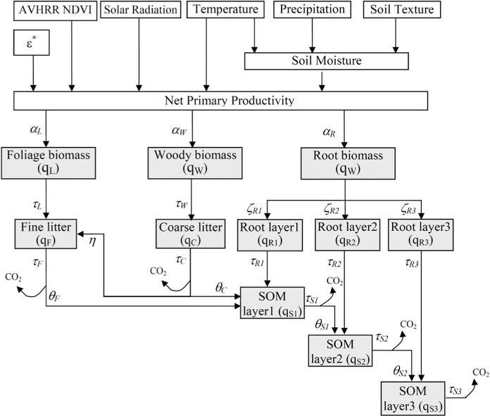
where f APAR is a fraction of photosynthetically active radiation (PAR) that is absorbed by vegetation and determined by using a linear relationship between f APAR and satellite-data derived normalised difference vegetation index (NDVI, Potter et al., 1993). Solar radiation is converted to PAR by multiplying 0.5. ɛ* is maximum potential light-use efficiency, and T ɛ and W ɛ are temperature and moisture scalars, respectively (see Supplementary material). The estimated NPP is allocated to plant tissues of leaves, stems and roots. Dead leaf, stem and root materials are transferred to respective litter compartments. Part of the litter C is respired and the remainder is converted into soil organic matter (SOM) pools. The relationships of C transfer among pools were simulated by the VAST algorithms. The first-order ordinary differential equations were applied to model C dynamics in the litter and soil organic C (SOC) pools (see Supplementary material, Barrett, 2002; Zhou and Luo, 2008). The model consists of two aboveground biomass pools, two litter pools, three root biomass pools and three soil C pools. Root biomass and soil C pools were divided into three soil layers (0–20, 20–50 and 50–100 cm) as in Barrett (2002) and Zhou and Luo (2008), instead of compartmentalised SOC according to decomposition rates as in most of the models (e.g., CENTURY, Parton et al., 1987; TECO, Luo et al., 2003). In this way, a one-to-one relationship was ensured between model state variables (especially for root biomass and SOC) and the respective observations obtained from the literature, which do not need extra mapping function as in Luo et al. (2003). We assumed that impacts of disturbances on C residence time were reflected by remote sensing data in NDVI. A schematic diagram of the TECO-R model is shown in Fig. 1.
Fig. 1.
Schematic diagram of the regional terrestrial ecosystem (TECO-R) model for inversion analysis of carbon residence time. NPP, which is modelled by maximum light-use efficiency (ɛ*) (CASA model), is allocated to plant tissues (leaf q L , stem q W and root ) based on allocation coefficients (α L , α W , α R ). Plant tissues enter into fine litter (q F ), coarse litter (q C ) and soil organic carbon pools (q S ) through litterfall. Decomposed litter releases part of the carbon to the atmosphere, and the rest transfers into the soil (θ C , θ F ). Through mechanical breakdown, part of the coarse litter becomes fine litter (η). To reflect the differences in soil profile, roots and soil organic carbon pools are divided into three layers (0–20, 20–50 and 50–100 cm). Each pool has an associated carbon residence time, τ k (k=1, 2, 3).
The C residence times in litter and SOC pools vary largely with both climatic and biotic factors (Schimel et al., 1994). To specify the biotic effects on the C residence times, eight vegetation types (ENF, evergreen needleleaf forest; DBF, deciduous broadleaf forest; MF, mixed forest; W, woodland; WG, wooded grassland; S, shrubland; G, grassland; and C, cropland) were set up in the conterminous USA based on the 1-km land cover classification by Hansen et al. (2000), and then the TECO-R model was used to estimate the parameters for each biome, separately. To specify the effects caused by spatial heterogeneity of climatic factors, temperature (T ɛ ) and moisture (W ɛ ) scalars were used to correct the site-specific C residence times The corrected residence times were called moisture and temperature corrected C residence times as follows:

The moisture scalar was estimated by monthly precipitation, potential evapotranspiration and soil moisture (Randerson et al., 1999). The temperature scalar was obtained directly from temperature data, as shown in the CENTURY soil-carbon model (see Supplementary material, Parton et al., 1987).
The estimated parameters by MCMC technique in this study included the maximum potential light-use efficiency (ɛ*), C allocation coefficients among pools and C residence times in individual plant and soil pools, totalling 22 parameters for each of the eight biomes (see Table 1 for the definition of all 22 parameters). Uncertainties of individual parameters and ecosystem C residence times were represented by SD and CV from Metropolis–Hastings (M–H) simulation (see Appendix S1 in Supplementary material). Ecosystem C residence times (τ E ) and their SD were aggregated from the allocation of coefficients and C residence time in the individual plant and soil pools over the conterminous USA using the following formula (Barrett, 2002):

where
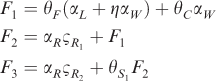
Ecosystem C uptake in the conterminous USA was estimated in forward modelling by using maximum likelihood estimates (MLEs) of parameters and mean changes in NPP from 1982 to 1998 as a C input by Hicke et al. (2002). Propagation of parameter uncertainties to modelled ecosystem C uptake was assessed through simulating C uptake for all 40 000 samples of C residence times and allocation coefficients from MCMC simulation and then calculating SDs and CVs in the conterminous USA.
2.2. Data sources
In this study, 13 observed data sets were used for the parameter estimation, including three NPP data sets (NPP in leaves, stems and roots), five biomass data sets (one for leaves, one for stems and three for roots in three soil layers; 0–20, 20–50 and 50–100 cm), two litter mass data set (fine and coarse litter mass) and three SOC data sets in the three soil layers (0–20, 20–50 and 50–100 cm) for each biome if any. Compared to the study by Zhou and Luo (2008), we added coarse litter and more fine litter data points. There were a total of 7828 observed data points, which contained 175 data points for litter (vs. seven data points in Zhou and Luo, 2008), 468 data points for NPP, 316 data points for biomass and 6869 data points for SOC. Spatial distribution and the detailed information of data points and their sources were documented in Appendix S2 in Supplementary material. Auxiliary data used in this study included: (1) the AVHRR-NDVI continental subsets of 8 km spatial resolution from 1982 to 1999 available from the Data and Information Services Center of Goddard Earth Science; (2) annual solar radiation produced by the NASA/Global Energy and Water Cycle Experiment with one-by-one degree spatial resolution; (3) monthly precipitation and temperature data sets with 4 km spatial resolution offered by the Spatial Climate Analysis Service; (4) soil texture data from State Soil Geographic Database (STATSGO) compiled by USDA Natural Resources Conservation Service; and (5) 1-km spatial resolution land cover data, containing eight vegetation types in the conterminous USA, derived from AVHRR using a decision tree classifier (Hansen et al., 2000). All those auxiliary data sets were resampled by ERDAS software with cubic convolution methods to a common projection (Lat–Long Projection) and spatial resolution (0.04°) (Smith and Brown, 1997).
2.3. Parameter estimation and uncertainties analysis
In the study, a Bayesian probabilistic inversion approach was employed in the TECO-R model to estimate C allocation coefficients and C residence times for each biome (a total of eight sets of parameters). A detailed description of the Bayes’ theorem was given by Xu et al. (2006) and McCarthy (2007). Below is a brief overview.
In the context of this study, we applied Bayes’ theorem to the C cycling. Specifically, the posterior PDF p(c∣Z) of C allocation coefficients and C residence times can be obtained from prior knowledge of parameters represented by a prior PDF p(c) and information contained in 13 data sets represented by a likelihood function p(Z∣c). To specify the biotic influences, Bayes’ theorem was applied for each of the eight biomes (ENF, DBF, MF, W, WG, S, G and C). Given one biome, we first specified the prior PDF p(c) by giving a set of limiting intervals for all parameters with uniform distribution (Table 1), and then constructed the likelihood function p(Z∣c) on the basis of the assumption that errors in the observed data followed Gaussian distributions. Parameter ranges were determined through a combination of literature values, knowledge of the system and prior information from Zhou and Luo's (2008) study for the optimal parameter values (Table 1). Initial C pools were set in 1987 and estimated by the method used in Luo et al. (2001) based on an initial steady-state C balance in the TECO model and experimental data at the start of this study. A partial likelihood function p i (Z∣c) was specified according to distributions of observation errors (e(t)) for data set m:

Table 1. Symbol and definition of parameters, their lower (LL) and upper limits (UL) and other constraints for inverse analysis. Unit is gC MJPAR −1 for ɛ * and years for carbon residence times. Allocation and partitioning coefficients are dimensionless.
where constant σ m 2 is the error variance of the mth data set, y nm is the nth observed data point in the mth data set, ŷ nm (x n , a) is the modelled value that corresponds to the observation y nm , N m is the total data points in the mth data set, x n is an auxiliary forcing vector that includes NDVI, solar radiation, air temperature, precipitation and soil texture in a spatial grid where the nth observation was made; and a is a vector consisting of 22 parameters: a = {ɛ * , α L , α W , α R , , , , τ L , τ W , θ F , θ C , η, , , , , , , , , , }, each of the parameters is defined in Table 1. An integrated likelihood function p(Z∣c), which consists of M (=13) partial likelihood functions p i (Z∣c), is defined to measure the deviations between modelled and observed values for all the data points in the 13 data sets as follows:

Therefore, with Bayes’ theorem, the PPDF of parameters is given by

Since Bayes’ theorem was applied to each of the eight biomes, eight sets of biome-specific values of parameter vector, a, were obtained in the study.
To draw samples from p(c∣Z), a M–H algorithm was employed to construct a PPDF of C residence time and C allocation coefficients on the basis of prior information of model parameters, model structure and the data sets. The M–H algorithm is a MCMC technique, which could obtain high-dimensional PDFs of random variables via a sampling procedure (Metropolis et al., 1953; Hastings, 1970; Gelfand and Smith, 1990). For each biome, 40 000 samples were generated by the five runs from the M–H simulation with an acceptance rate of about 30–40% for the newly generated samples when the five runs converged as indicated by the G-R statistics (see Supplementary material). Marginal distribution, MLEs, means, SD and CV of C residence time and allocation coefficients were calculated from simulated 40 000 samples to assess the uncertainties of parameters (see Appendix S1 for a detailed description of the M–H algorithm, as well as an estimate of maximum likelihood estimators (MLEs), means and cross-correlations between parameters in Supplementary material).
2.4. Carbon uptake and uncertainties analysis
The MLEs of parameter values estimated from M–H simulation together with the corresponding C pool sizes in the inverse analysis were used in forward modelling to simulate ecosystem C uptake. In addition to C residence time, NPP is another key factor that determines the capacity of an ecosystem to absorb C (Luo et al., 2003). Hicke et al. (2002) estimated that the averaged NPP increase was 1.83 g C m−2 yr−1 (i.e., 0.5% per year) from 1982 to 1998 by remote sensing in the conterminous USA but the trend in NPP changes varied with ecosystems. We applied the actual spatial pattern of NPP changes from Hicke et al. (2002) to quantify C uptake for each spatial grid at a yearly time step. Therefore, the spatial difference of C uptake potential was caused by both the spatial pattern of C residence times and NPP changes. In our study, to focus on these two factors (i.e., NPP changes and C residence times) in influencing C uptake, we assumed that impacts of disturbance and environmental factors (e.g., temperature) on C uptake were reflected by remote sensing data in NDVI.
Uncertainties of terrestrial C uptake were assessed by the SDs and coefficients of variation (CVs). We used 40 000 samples of C residence times and allocation coefficients estimated from M–H simulation as expressed by PPDFs p(c∣Z) for each biome to simulate ecosystem C uptake and assess propagation of the parameter uncertainties in forward modelling as described above. The forward model simulation for ecosystem C uptake was made over 50 yr from 1987 to 2036. The SDs and CVs were calculated from the 40 000 data sets of ecosystem C uptake in the conterminous USA.
3. Results
3.1. Comparison between modelled and observed data sets
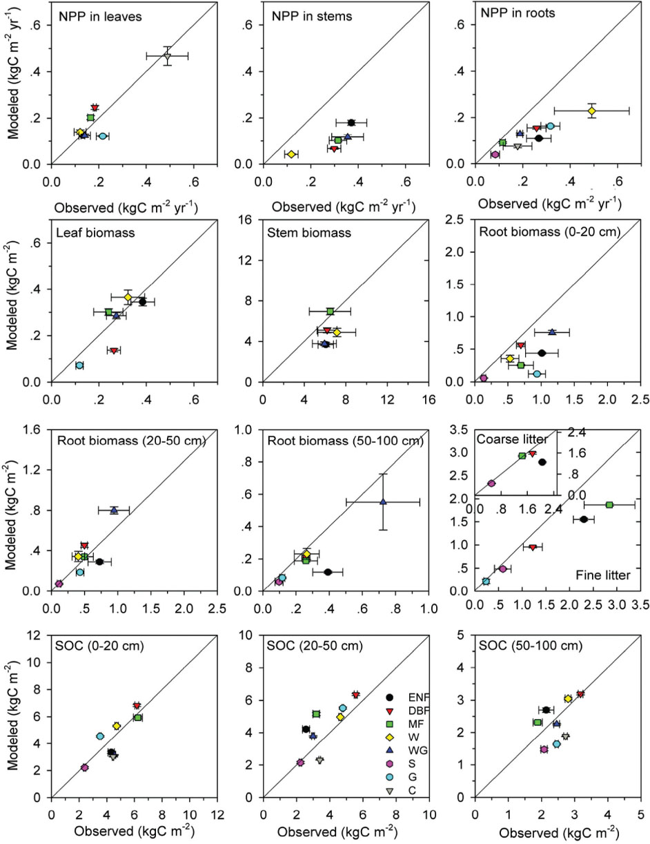
To evaluate the validity of the inverse analysis method, it is important to compare the values between modelled and observed data sets. This study used the 13 observed multi-site data sets and multiple sources of information to constrain the parameters for each biome (totally eight biomes), which may reduce uncertainty. The TECO-R model with the Bayesian inversion reasonably simulated C fluxes and pools in the conterminous USA, which were closely related to the corresponding observed data sets (Fig. 2). There were a few cases where modelled values deviated from observations. For example, the simulated NPP in roots and stems, and root biomass in 0–20 cm soil layer were largely underestimated compared to the observed data (Fig. 2).
Fig. 2.
Comparisons between modelled and observed data lumped by each biome for 13 data sets. Biomes: ENF, evergreen needleleaf forest; DBF, deciduous broadleaf forest; MF, mixed forest; W, woodland; WG, wooded grassland; S, shrubland; G, grassland; and C, cropland. Unit with dimensions is not shown.
3.2. Estimated C residence times and allocation coefficients
The histograms of 40 000 samples generated by the five runs from the M–H simulation are shown in Fig. 3 for ENF and in Fig. 4 for G, representing forest and non-forest biomes, respectively, when the five runs converged as indicated by the G-R statistics (=1, data not shown). For all eight biomes, most of the parameters are nearly Gaussian distributed but with considerable differences in their variability. Parameters ɛ * , α L , α W , α R , , and were well constrained with steep peaks of frequencies (Figs. 3 and 4). In contrast, parameters θ F , θ C , , , η and were constrained to some degree but with considerably spread posterior PDFs. Other parameters contain intermediate information on parameter constraint compared to those well and loosely constrained (Figs. 3 and 4). Several parameters (e.g., τ W , ) were well constrained by some biomes but not by others, probably due to the limitation of available data.
Fig. 3.
Inversion results showing the histograms of 22 estimated parameters and cost function with 40 000 samples from M–H simulation for evergreen needleleaf forest (ENF). See Table 1 for parameter abbreviation. Unit with dimensions is not shown.
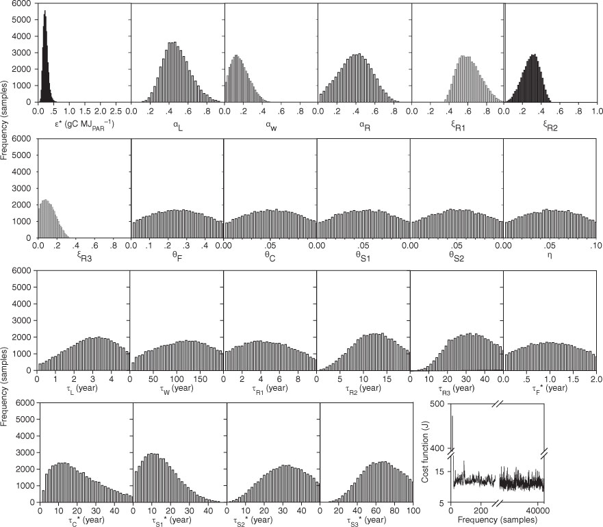
Fig. 4.
Inversion results showing the histograms of 17 estimated parameters and cost function with 40 000 samples from M–H simulation for Grassland. See Table 1 for parameter abbreviation. Unit with dimensions is not shown.
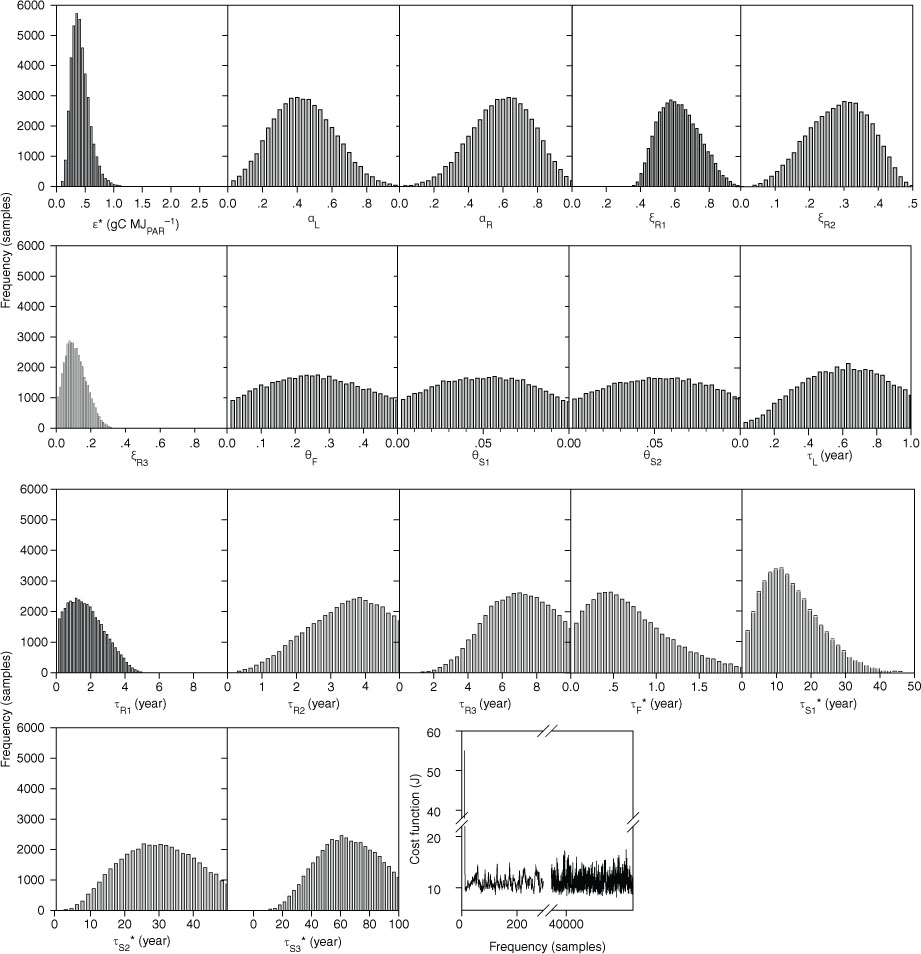
In performing a simultaneous optimisation on 22 parameters, which provides an ensemble of parameter sets, it is likely to have parameter correlations due to tradeoffs between the parameters pairs. Our cross-correlation analysis showed that more than 85% of correlations between parameters, ∣corr∣, were below 0.2 and >90% were below 0.3 (Appendix S3 in Supplementary material). High ∣corr∣ values (>0.4) mainly resulted from equality constraints (e.g., α L +α W +α R =1). In addition, allocation of NPP to wood (α W ) was directly related to C residence times of wood (τ W ) and coarse litter (τ C ), resulting in high ∣corr∣ values with a range of 0.4–0.7 depending on the biomes.
The MLEs are the parameter values corresponding to the peaks of their marginal distributions (Figs. 3 and 4). The estimated maximum potential light-use efficiencies (ɛ*) varied largely with vegetation types (Fig. 5a), being high in cropland (0.71±0.20 g C MJPAR −1) and being low in ENF (0.23±0.08 g C MJPAR −1). The S has the largest variability (CV=119%) with a ɛ* value of 0.47±0.56 g C MJPAR −1. The ɛ* values for DBF, G, MF, W and WG were similar, ranging from 0.30 to 0.41 g C MJPAR −1 (Fig. 5a). Our estimated maximum potential light-use efficiency of cropland was within the range from 0.41 to 0.94 g C MJPAR −1 given by Lobell et al. (2002).
Fig. 5.
MLEs or means of estimated parameters for eight biomes. Error bars represent standard deviations (SDs) of parameters calculated from 40 000 samples of M–H simulation. Parameters θS1 and θS2 were not shown due to their consistence between biomes (0.05±0.03). See Fig. 2 for biome abbreviations and Table 1 for parameter abbreviations.
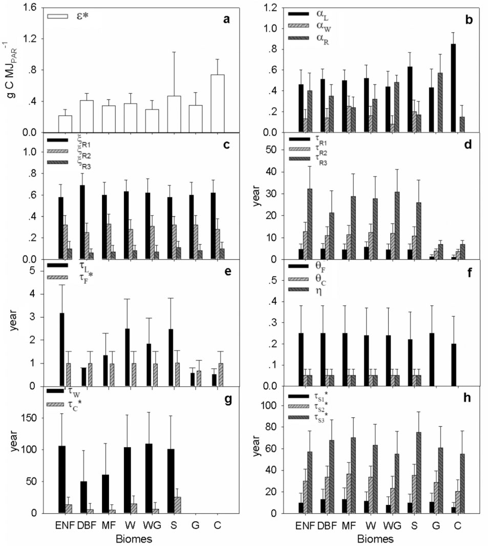
Allocation coefficients of NPP to leaves, stems and roots also varied with biomes (Fig. 5b). C allocation to leaves was relatively higher for the cropland (79±11%) and S (60±14%) than the other biomes, which had similar C allocation coefficients from 42±18% (G) to 52±10% (MF). The C allocation of NPP to stems ranged from 12±8% (WG) to 23±10% (MF). Accordingly, there were relatively lower C allocation to roots for MF, S, and cropland (20±13 to 24±10%) and higher C allocation for G (58±18%) and WG (44±7%). For the two non-forest biomes (G and cropland), which allocated C only to leaves and roots, G allocated much more C into roots (58±18%) than cropland did (21±11%). The results were similar to the findings from Bradford et al. (2005), showing cropland allocated 28% of NPP to roots, much lower than G. Vegetation types did not significantly affect the allocation coefficients of roots to three soil layers (0–20, 20–50 and 50–100 cm) (Fig. 5c).
In DBF, G and cropland (0.50±0.27 to 0.61±0.02 yr), the C residence times of leave (τ L ) were much lower than those in other biomes (1.58±0.97 to 2.82±1.22 yr, Fig. 5e). However, the C residence times of wood (τ W ) did not vary largely with biomes (78.8±48.8 to 109.3±52.4 yr) but they appeared in high variability (CV=46–62%, Fig. 5g). The root residence times varied from 4.46±2.60 to 5.37±2.38 yr in top soil layer, 11.44±1.23 to 12.38±3.92 yr in middle soil layer and 27.12±10.1 to 31.1±10.3 yr in deep soil layer for the forests, W and S (Fig. 5d). The G and cropland had much lower root residence times for all three layers than other biomes (Fig. 5d). The temperature- and moisture-corrected C residence times of litter and SOC showed considerable uncertainties with large SDs (Fig. 5e, g, h). The C residence times of fine litter (τ F *) were only well constrained for G, showing the lowest value (Fig. 5e). The C residence times of coarse litter (τ C *) were relatively lower for DBF, MF and WG with a range from 11.1±8.8 to 13.9±10.4 yr than those for ENF, W and S (19.3±11.9 to 25.7±13.1 yr). The values of SOC residence times were much higher than those of litter, ranging from 7.48±4.86 to 17.3±10.3 yr for the top soil layer, from 23.5±10.7 to 32.8±10.4 yr for the middle soil layer, and from 56.7±21.4 to 67.3±18.8 yr for the bottom layer, but they did not vary largely with biomes. C partitioning coefficients also did not vary with biomes but with large variability (CV>50%).
3.3. Spatial patterns of ecosystem C residence times
The C residence time of the whole ecosystem varied highly with locations (or ecosystems) in the conterminous USA, ranging from about 10 yr in some cropland grids to 180 yr in some S grids (Fig. 6a). However, most values fell between 15 and 90 yr. The averaged C residence time of the whole conterminous USA was 56.8 yr. The west regions had higher C residence time, while the central and east regions showed lower values. The SDs of the ecosystem C residence time for each grid were shown in Fig. 6b, ranging from 1 to 32 yr, with most values between 2 and 15 yr. The averaged SD of ecosystem C residence time was 8.8 yr for the conterminous USA. As shown by the coefficients of variation (CV=SD/mean), large uncertainties appeared in southern USA (CV=14–22%) and small uncertainties in the central (CV=5–10%, Fig. 6c).
Fig. 6.
Spatial patterns of ecosystem carbon residence times (a), its standard deviation (SD, b) and coefficient of variation (CV=SD/mean, c) in terrestrial ecosystems of the conterminous USA.
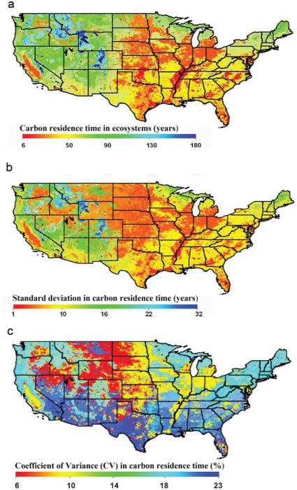
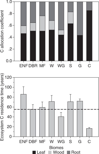
Among all eight biomes, the cropland had the lowest C residence time (16.6±1.8, Fig. 7b) due to the lack of long residence wood tissues and coarse litter. WG also showed the relative low C residence time because of the low allocation of wood tissue from NPP (40.5±8.5, Fig. 7a). The ENF showed the highest C residence times of 85.9 years, probably due to the low temperature in this area. The other biomes had C residence times between 55.9±9.7 and 72.1±4.1 yr. Along the latitude, C residence time displayed a strong positive correlation (Appendix S4 in Supplementary material, R 2=0.91), suggesting that temperature could be one of the most important factors in influencing C residence times.
Fig. 7.
Carbon allocation coefficients (a) and the averaged ecosystem C residence time (b) for eight biomes. See Fig. 2 for biomes abbreviation. Horizontal dash line represents the average ecosystem C residence time in the conterminous USA. Error bars represent standard deviation.
3.4. Carbon uptake in soil and ecosystems
When the actual, spatially heterogeneous NPP changes from Hicke et al. (2002) was applied to each spatial grid in the forwarding model, the estimated ecosystem C uptake showed large variability with a range from −60 to 140 g C m−2 yr−1 within the 50 yr. The southeast regions had higher C uptake, possibly due to the relatively higher values of both NPP increases and C residence times (Fig. 8a and Appendix S5). The Central Plains also had high C uptake, which may mainly result from the highest NPP increase in the conterminous USA. But ecosystem C release occurred in some southwest regions because of decreased NPP (Fig. 8a and Appendix S5). The estimated total C uptake in the conterminous USA was 0.20±0.06 Pg C yr−1. For each biome, the large C uptake appeared in ENF, MF, cropland and G, while S did not contribute C uptake in the conterminous USA (Fig. 9). Among the ecosystem C uptake, soil contributed about 50% of C uptake. G and cropland had the relatively higher proportions of soil C uptake (51–82%) than forests and Ws (25–49%) (Figs. 8c and 9).
Fig. 8.
The potential of ecosystems C uptakes (a), their coefficient of variance (b) and proportion of soil to ecosystem C uptake in the conterminous USA under the actual NPP increases from Hicke et al. (2002). The positive value means C sink while the negative value mean C source.
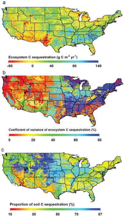
Fig. 9.
Yearly ecosystem and soil C uptake in different biomes under the actual NPP increases from Hicke et al. (2002). Error bars represent standard deviation (SD).
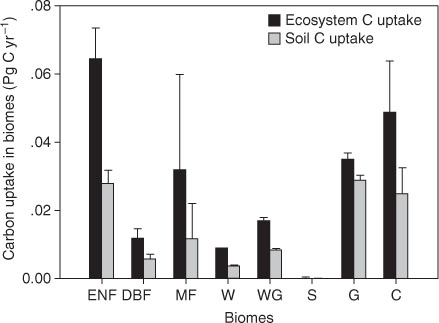
The coefficients of variance (CVs) of ecosystem C uptake were higher in central and eastern USA with a range from 50 to 80% than other regions from 0 to 40% (Fig. 8b). Both high C residence times and large increases in NPP may mainly lead to high variability in ecosystem C uptake in these regions. The ENF, MF and cropland displayed large uncertainties with high SDs (Fig. 9).
4. Discussion
The results from atmospheric inversion methods have substantially improved our understanding on the dynamics of the global and regional C cycle over several decades (Kaminski et al., 2002; Rayner et al., 2005; Prihodko et al., 2008). Meanwhile, the atmospheric inversion can be greatly complemented by the application of multiple-constraint data assimilation with ecological observations in predictive understanding of ecosystem C uptake (Barrett, 2002; Wang and Barrett, 2003). In this study, the multiple-constraint approach with Bayesian inversion of a regional terrestrial ecosystem model (TECO-R) worked well to optimise C residence times and assess their uncertainties with SD and CV. The method also provided information on parameter correlations. Such information on uncertainties of C residence time is crucial for understanding the degree of confidence we can have on model predictions of the global terrestrial C balance.
4.1. Method comparisons on estimated carbon residence times
Comparisons between modelled and observed data are essential to evaluate the validity of the inverse analysis method. When most of the modelled values were closely related to the corresponding observed data, the TECO-R model simulated the lower values for the NPP in roots and stems, and root biomass in 0–20 cm soil layer compared to the observed ones (Fig. 2). The large underestimation is probably due to both model assumptions and observation errors. The model assumed that stem and root allocation coefficients depended on leaf allocation coefficients (α L +α W +α R =1), and the residence times of roots were on a scale of years. We allowed the model to search for root residence times within ranges of 0–10, 0–20 and 0–50 yr in three soil layers (0–20, 20–50 and 50–100 cm), respectively. Generally, the root residence times of deep soil layers (20–50 and 50–100) may be larger than those of soil surface. The wide lower ranges (close to 0) for the two deep soil layers may underestimate root residence times. On the other hand, the observed root NPP and biomass were estimated from a variety of methods (e.g., ingrowth cores, minirhizotron and allometry; Jackson et al., 1996) and stem NPP was usually indirectly estimated from diameters at the breast height (DBH, DeLucia et al., 1999), possibly resulting in large errors in different locations. In addition, the tradeoff of estimated parameter values under the integrated cost function for all data sets minimised the total deviation possibly at expense of stem and root NPP.
Using Bayesian inversion technique in this study, most of the estimated optimal C residence times were similar to those from Zhou and Luo (2008) using generic algorithm (GA), although there were the less observed data sets in Zhou and Luo (2008) (i.e., no coarse litter and only seven fine litter data points). C residence times of leaves for forests and Ws ranged from 0.78 to 3.17 yr, which were comparable to those estimated by observed stocks and fluxes with 1.64 yr for Ws and 2.32 yr for forests (Cannell, 1982; DeAngelis et al., 1997). The C residence times of wood ranged from 78.8 to 109.3 yr similar to those estimated from C balance and radiocarbon dating methods (Cannell, 1982; Turner, 1984; DeAngelis et al., 1997). The estimated temperature- and moisture-corrected residence times of fine litter were from 0.67 to 1.0 yr (Fig. 5), which were very close to the means from meta-analysis by Silver and Miya (2001) and Zhang et al. (2008). The estimated residence times of coarse litter were from 5.0 to 25.7 yr (Fig. 5), well within the range (2.3–33 yr) summarised from coarse-wood decomposition experiments for deciduous and coniferous species in the eastern USA (Todd and Hanson, 2003). The estimated C residence times of roots were similar to those from the other two inverse analysis by Genetic Algorithm (GA) in Australia and USA (Barrett, 2002; Zhou and Luo, 2008), but were much higher than the experimental estimations (Gill and Jackson, 2000). The discrepancy between modelling and experiments may result from the differences of root representatives for soil layers, time scales and the methods (Jackson et al., 1996). The estimated residence times of SOC increased with soil depth, having a range of 5.53–13.32 yr for the top soil layer, 20.35–36.73 yr for the middle soil and 55.01–75.34 yr for the bottom soil (Fig. 5), which were comparable from only a few studies at different soil layers (Jenkinson et al., 1999; Fontaine et al., 2007). However, most of the experimental studies showed larger ranges from several years to thousands of years when only the surface soil or one combined soil layer was used (Jenkinson et al., 1999; Garten and Hanson, 2006).
To facilitate parameter estimation in this study, we divided SOC and root biomass into three soil layers (0–20, 20–50 and 50–100 cm) as by Barrett (2002) and Zhou and Luo (2008), instead of compartmentalised SOC (i.e., fast, slow and passive) according to decomposition rates as well as fine root and coarse root compartments in most of the models (e.g., CENTURY, Parton et al., 1987; TECO, Luo et al., 2003). In this way, a one-to-one relationship was ensured between modelled and observed root biomass and SOC, and the models do not need extra mapping functions as by Luo et al. (2003). In the process-based models, the conceptual compartmentalised SOC generally cannot be measured directly. The experimentally extractable soil C pools (e.g., labile and the remaining recalcitrant pools) cannot simply represent the conceptual C pools in the mechanistic models. This highlights the need for a comprehensive representation of belowground C-pools in the process models (including deep soil C) in order to achieve unbiased parameter estimates (Barrett, 2002).
The relatively fast turnover of ecosystem C appeared in the east and central regions, largely resulting from the cropland and G due to the lack of long-residence wood tissues and coarse litter (Figs. 6a and 7b). In the west regions, forests and Ws are in the mountainous regions with high residence times (Fig. 7b). In addition, our results that C residence times correlated positively with the latitude (Appendix S4, R 2=0.91) suggested that temperature may be a key factor in influencing C residence time. The estimated aggregate ecosystem C residence time in the conterminous USA was 56.8 yr, which represented an upper limit of the global average C residence time (26–60 yr) as estimated by various experimental and modelling approaches (Raich and Schlesinger, 1992; Randerson et al., 1999; Thompson and Randerson, 1999), but was lower than the estimation by Barrett (2002) in Australia (78 yr). The relatively high ecosystem C residence time in the conterminous USA compared to the global average one mainly resulted from the inclusion of deep C in the soil profile (0–100 cm).
4.2. Uncertainties in C residence times
Unlike the methods of uncertainties analysis by varying one parameter at a time (Knorr, 2000; El Maayar et al., 2002), the probabilistic inversion can estimate the probability of uncertain parameters and state variables (McCarthy, 2007). The Bayesian approach constructs parameter distributions and assesses parameter uncertainties by quantifying MLEs, means, SDs, and CVs, and offers much richer information contained in data, model structure and prior knowledge on parameters than the deterministic inversion (Raupach et al., 2005; Xu et al., 2006). Our results showed that posterior PDFs of most of the parameters are nearly Gaussian distributed but with considerably different variability, which were largely improved in comparison with the prior uniform distribution (Figs. 3 and 4). The MLEs of relatively well constrained parameters ɛ * , α L , α W , α R , , and were equivalent to optimal estimates from deterministic inversion using the least squares method (Tarantola, 1987; Raupach et al., 2005), which are generally in good agreement with those by GA in Zhou and Luo (2008). A very large set of various observations, especially NPP and biomass in leaves, stems and roots, is advantageous to constrain these allocation coefficients of C from NPP.
The parameters θ F , θ C , , , η and were constrained to some degree but with considerably spread posterior PDFs. Their large uncertainties were probably due to either the lack of experimental data or the mismatch of timescales between the available data and the parameters to be estimated. For example, the lack of microbial biomass, respiration and other data probably resulted in low constraints of parameters related to litter and SOC dynamics (Xu et al., 2006). Because of the mismatch between timescales for observation of vegetation change and parameters, little is known about the dynamics of terrestrial ecosystems over long temporal scales (Wiegand and Milton, 1996). In addition, parameter correlations (e.g., α W –τ W or τ C ) may also result in large uncertainties in C residence times (Appendix S3). Xu et al. (2006) found that reduced measurement errors led to substantially reduced uncertainties of estimated parameters, suggesting that error magnitudes in observations may be one of the factors in determining parameter uncertainties. Prior information about parameter space has been suggested to be another source of parameter uncertainties (Spear et al., 1994). When we expanded prior ranges of these parameters (i.e., increased upper limit), their histograms, however, did not show statistically significant changes, similar to the finding from Xu et al. (2006).
Parameters , , and were relatively well constrained by 13 data sets (Figs. 3 and 4), probably due to a large number of data sets on roots and soil C (Appendix 2–3). The parameters representing long C residence times from deep old SOC pools (i.e., and ) can be further constrained by long-term observations or data sets that characterise long-term processes, such as those from C isotope studies (Randerson et al., 2002; Scholze et al., 2008).
Ecosystem C residence times in the conterminous USA showed large spatial variability and uncertainties (Figs. 6b, c). Uncertainties of ecosystem C residence times as indicated by CV were high in southern USA with a range of 14–22% and low in the central area (6–12%, Fig. 6c). The spatial distribution of uncertainties in the conterminous USA may be attributable to either the lack of experimental data or the mismatch of timescales between the available data and the estimated parameters as well as environmental conditions. CVs of ecosystem C residence times were similar with a range from 17.2 to 21.0% except G (6.0%) and cropland (10.9%, Fig. 7b). Low uncertainties of C residence times in the G and cropland greatly resulted from availability of large volumes of data and relatively evenly distributed environmental conditions over space, particularly in croplands, compared to those in forests and W.
4.3. Estimated ecosystem C uptake and its uncertainties
Driven by NPP changes from 1982 to 1998 as estimated by Hicke et al. (2002), total C uptake estimated by the Bayesian approach was 0.20±0.06 Pg C yr−1 in the conterminous USA. The estimate is comparable to the one by Houghton et al. (1999) with a value of 0.15–0.35 Pg C yr−1 based on the analysis of historical data on land use and land cover changes as well as inventory estimate (0.30 Pg C yr−1, Birdsey and Heath, 1995). However, this estimate is larger than an ensemble of three models (Biome-BGC, Century and TEM) with a value of 0.08 Pg C yr−1 (Schimel et al., 2000) but smaller than C sink from atmospheric inversion with a range from 0.30 to 0.58 Pg C yr−1 (Pacala et al., 2001).
Ecosystem C uptake is largely determined by both ecosystem C residence time and C input (Luo et al., 2003). Our modelling results show that both forest and non-forest ecosystems are potentially important to sequester C in the conterminous USA (Fig. 8a and 9). The spatial pattern of ecosystem C uptake was closely related to the greenness map from U.S. Geological Survey (USGS) in the summer (http://ivm.cr.usgs.gov/). The most important forests for C uptake were ENF and MF, which were located in the southeast regions. This may be attributed to the young stand age of pine plantations (Sheffield and Dickson, 1998) and the immature hardwood forests (Brown et al., 1997). Currently, many of the pine stands in southern states have large potentials to increase productivity with intensive management (Allen et al., 1990). Interestingly, our results suggested that the substantial amounts of carbon (42% of the total) were sequestered in the G and cropland, which was comparable to the study by Pacala et al. (2001) with atmospheric inverse analysis. The substantial C uptake in the G and cropland largely resulted from their large areas, the Conservation Reserve Program (i.e., conversion of unproductive croplands to perennial G), expanded uses of no-till agriculture and improved productivity due to new plant varieties and increased fertiliser inputs (Houghton et al., 1999; Pacala et al., 2001; Lobell et al., 2002). In addition, disturbance and land management are important components of terrestrial C balance. In this study, we simply assumed that impacts of disturbance, land management and environmental factors on C residence time and uptake were reflected by remote sensing data in NDVI.
It is evident that large uncertainties remain in our assessment of terrestrial C uptake on the regional and global scales (Schimel et al., 2000; Pacala et al., 2001). Our results show large uncertainties with high CV in continental C storage, especially in central and eastern USA (Fig. 8b). The large uncertainties in C uptake could result from high spatial variability in initial NPP values, C residence times, or both (Fig. 6a and Appendix S5). To separate sources of uncertainties, we applied a uniformed NPP increase of 1.83 g C m−2 yr−1 (i.e., the averaged NPP increase in the conterminous USA from Hicke et al. (2002)) to quantify uncertainties of ecosystem C uptake. Our results suggest that the main source of uncertainties in C uptake was from spatial variability in C residence times (data not shown). In addition, the initial condition of NPP was another source of uncertainties. In the central and eastern USA, high variability in initial NPP and median variability in ecosystem residence time were combined to contribute to the large uncertainties (Fig. 7a). Therefore, uncertainties of ecosystem C uptake were strongly influenced by variability in C residence times and initial NPP values. Uncertainties in C uptake also varied with biomes (Fig. 9). The ENF, MF and cropland thus displayed larger uncertainties than the other biomes (Fig. 9). Besides those reasons discussed above, one additional cause of the high uncertainties in forest C uptake is scarce observations in mountainous regions where forests grow.
In this study, the 40 000 samples of posterior parameters were used to assess the regional uncertainty in terrestrial C uptake for the conterminous US. However, it is impractical with such a large size of ensemble simulations to assess the uncertainty in the global models (e.g., Community Land Model - CLM), especially with 3-D earth system models. To reduce the computational cost for assessing the regional uncertainty, we randomly selected 5000 samples to test whether a subset of posterior parameters could represent all parameters or not. We found that the results from these two sets of posterior parameters were similar (data not shown). We can thus use a subset of posterior parameters to reduce the computational cost in assessing the uncertainty for global models.
This study focuses on the uncertainties in process-based terrestrial ecosystem models due to parameter uncertainties, and aims at providing quantitative information about the confidence in model results. Future steps toward a quantitative assessment of uncertainties in modelling terrestrial ecosystem dynamics will need to account for uncertainties related to model assumptions and to consider driving factors of climate change such as warming, elevated CO2, altered precipitation, and land use change and N deposition. In addition, investigation and mapping of disturbances are important to quantify C uptake in the conterminous USA, particularly in the human-impacted ecosystems. Long-term remote-sensing data sets may be important to provide estimates of disturbance that could also be assimilated into a model. An important improvement in our understanding of uncertainties might be obtained by the combination of long-term experiments with well-documented time series data, such as net ecosystem exchange by eddy covariance, NPP, plant biomass, SOC and by the integration of the results with ecosystem modelling in a multiple-constraint framework.
5. Conclusions
Terrestrial ecosystems play a significant role for CO2 uptake in global C cycling budget. The capacity of ecosystem C storage is largely determined by C residence time in plants and soil. However, C residence time is a large source of uncertainties in the present understanding of the global C cycle. To reduce its uncertainties and improve prediction from C-cycle models, quantifying C residence times and assessing its uncertainties becomes paramount. In this study, we applied Bayesian approach with a M–H algorithm to a regional model (TECO-R) to quantify optimal C residence times and assess their uncertainties with marginal distribution, SDs and CVs in the conterminous USA based on 13 data sets. Our results showed that most of the parameters are nearly Gaussian distributed but with considerably different variability. The parameters with large variability may be related to low availability of experimental data or a mismatch of timescales. The cross-correlations of parameters (corr) illustrated that more than 85% of the ∣corr∣ values were below 0.20, and the high ∣corr∣ values mainly resulted from equality constraints. With MLEs of estimated parameters, the estimated average ecosystem C residence time was 56.8±8.8 yr with a range from 16.6±1.8 (cropland) to 85.9±15.3 yr (ENF). Ecosystem C residence times and SDs have highly spatial heterogeneity and their values depend on vegetation types and climate conditions. Large uncertainties (i.e., high CV) in estimated C residence times appeared in the southern and eastern USA. Under the driving force of NPP changes from 1982 to 1998, the forward modelling estimated that terrestrial ecosystems in the conterminous USA would absorb about 0.20±0.06 Pg C yr−1. Uncertainties of ecosystem C uptake were strongly influenced by variability in C residence times and initial NPP values. The Bayesian approach developed here is powerful for assimilating multiple source of information to constrain parameter estimation and assess uncertainties in model prediction.
6. Acknowledgements
The authors thank the two anonymous reviewers for the insightful comments on the manuscript. This research was financially supported by ‘Thousand Young Talents Program’ in China and The Program for Professor of Special Appointment (Eastern Scholar) at Shanghai Institutions of Higher Learning as well as US National Science Foundation (NSF) under DEB 0078325 and DEB 0444518, and by the Terrestrial Carbon Program at the Office of Science, US Department of Energy, Grants No.: DE-FG03-99ER62800 and DE-FG02-006ER64317.