Fig. 1.
Liquid, solid and total precipitation in the Arctic region (60 °N to 90 °N) from the operational ECMWF analyses. Dashed lines represent the extreme values reached during the 6-yr simulation.
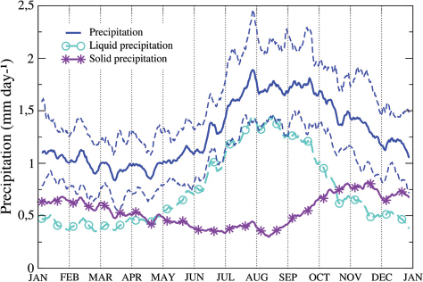
Table 1. Global burden (Tg[S] for sulphate, Tg for BC and dust) and residence time (days) of sulphate, BC and mineral dust, as simulated over the year 2000 by MOCAGE with the old and the new parameterisations of scavenging (columns Param_old and Param_new) and results from the AEROCOM intercomparison exercise (Textor et al., 2006; mean values of the 16 global chemical transport models in the column Aerocom mean, with range of values in square brackets)
[i] Note: Contrary to the old parameterisation, the new one includes scavenging by ice droplets and a 0.2 lower boundary for sulphate transfer coefficient ɛ. Values in brackets in the Param_old columns refer to a simulation without ice droplets scavenging but using a lower 0.2 boundary for ɛ sulphate.
Fig. 2.
Monthly mean of the atmospheric sulphate surface concentration (µg[S] m−3) simulated by MOCAGE (red) and observed at EMEP stations (blue). Bottom right: the map displays the location of the stations and the 2000–2005 averaged observed sulphate concentrations.
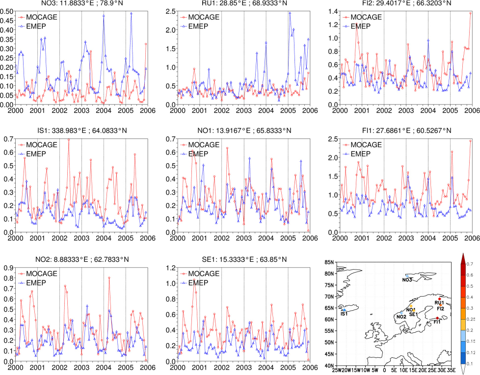
Fig. 3.
Monthly mean of the atmospheric sulphate surface concentration (µg[S] m−3) simulated by MOCAGE (red) and observed at Denali national Park, Barrow and Alert (blue). Bottom right: the map displays the location of the stations and the 2000–2005 averaged observed BC concentrations.
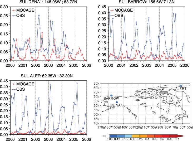
Fig. 4.
Monthly mean of the atmospheric black carbon (BC) surface concentration (µg m−3) simulated by MOCAGE (red) and observed at EMEP stations (blue). Bottom right, the map displays the location of the stations and the 2000–2005 averaged observed BC concentrations.
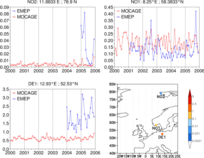
Fig. 5.
Monthly mean of the atmospheric BC surface concentration (µg m−3) simulated by MOCAGE (red) and observed at Denali national Park, Barrow and Alert (blue). Bottom right: the map displays the location of the stations and the 2000–2005 averaged observed BC concentrations.
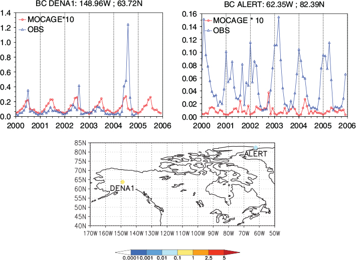
Fig. 6.
Left: Burden, sinks, sources and residence time of sulphate averaged over the Arctic domain. The average is a weekly moving average of the annual cycle over 2000–2005; dashed lines represent the extreme values reached during the 6-yr simulation. Right, top: sulphate burden (mg[S] m−2, 2000–2005 seasonal average); right, bottom: zonal mean of sulphate concentration (µg[S] m−3, 2000–2005 seasonal average, pressure levels in hPa on the vertical axis). All graphs show MOCAGE model outputs.
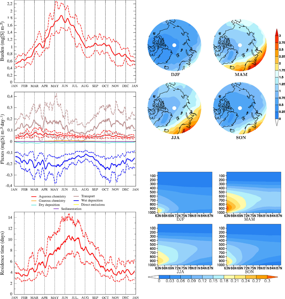
Fig. 7.
Left: Burden, sinks, sources and residence time of BC averaged over the Arctic domain. The average is a weekly moving average of the annual cycle over 2000–2005. Dashed lines represent the extreme values reached during the 6-yr simulation. Right, top: BC burden (mg m−2, 2000–2005 seasonal average); right, bottom: zonal mean of BC concentration (µg m−3, 2000–2005 seasonal average, pressure levels in hPa on the vertical axis). All graphs show MOCAGE model outputs.
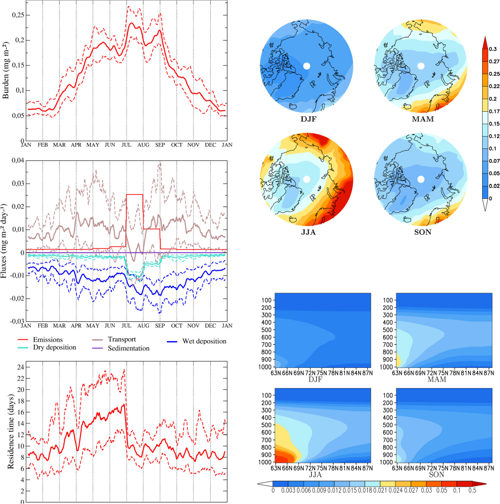
Fig. 8.
Left: Burden, sinks, sources and residence time of mineral dust averaged over the Arctic domain. Average is a weekly moving average of the annual cycle over 2000–2005. Dashed lines represent the extreme values reached during the 6-yr simulation. Right, top: dust burden (mg m−2, 2000–2005 seasonal average); right, bottom: zonal mean of dust concentration (µg m−3, 2000–2005 seasonal average, pressure levels in hPa on the vertical axis). All graphs show MOCAGE model outputs.
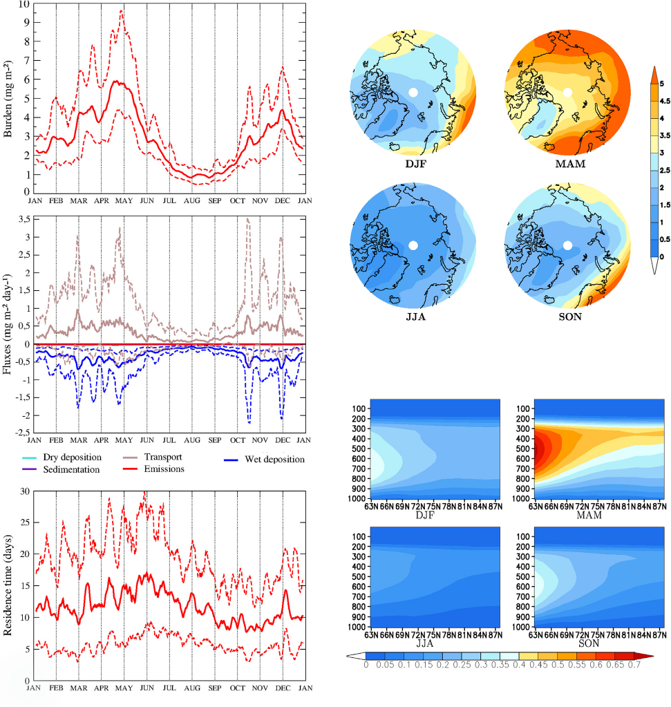
Fig. 9.
Sulphate, (BC) and mineral dust burden averaged over March–May 2001 (left) and 2004 (right). Mean burden values (M) and Residence Time are indicated under each figure for each aerosol and year.
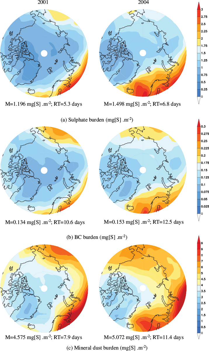
Fig. 10.
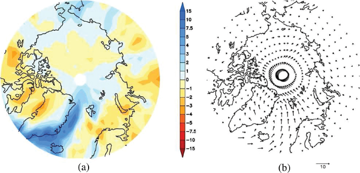
Precipitation (a, mm d−1) and wind (b, m s−1) differences between MAM 2004 and MAM 2001.