
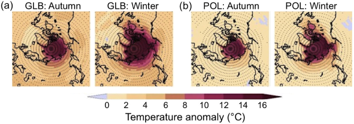
Fig. 1
Surface warming in polar region due to different climate forcings. Change of surface air temperature (°C) in autumn and winter for a sea-ice-free period relative to control climate computed with (a) global (GLB) and (b) polar forcing (POL). Stippled areas represent statistically significant changes with confidence level 95%.
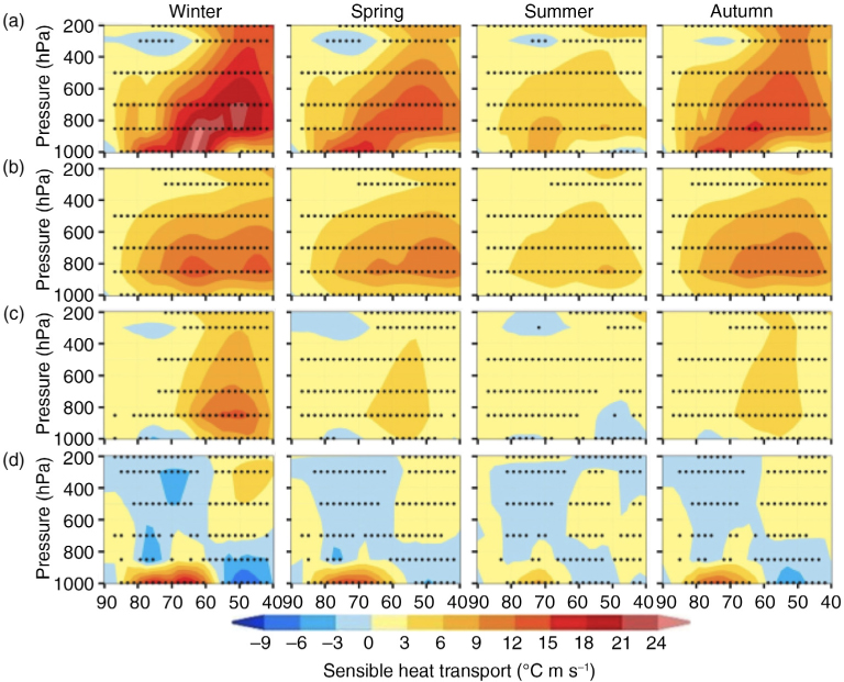
Fig. 2
Meridional heat transport by the atmosphere in control-run climate. Seasonal zonally averaged transport of sensible heat (°C·m·s−1) from 40 to 90°N computed in an atmospheric model with prescribed SIC, SIT and SST for the control period (1980–1989). Here the total heat transport (a) is decomposed into transport by transient eddies (b), large-scale stationary eddies (c) and mean meridional circulation (d). Northward transport is positive, and southward is negative. Stippled areas indicate that the absolute value of the transport is larger than its SD.
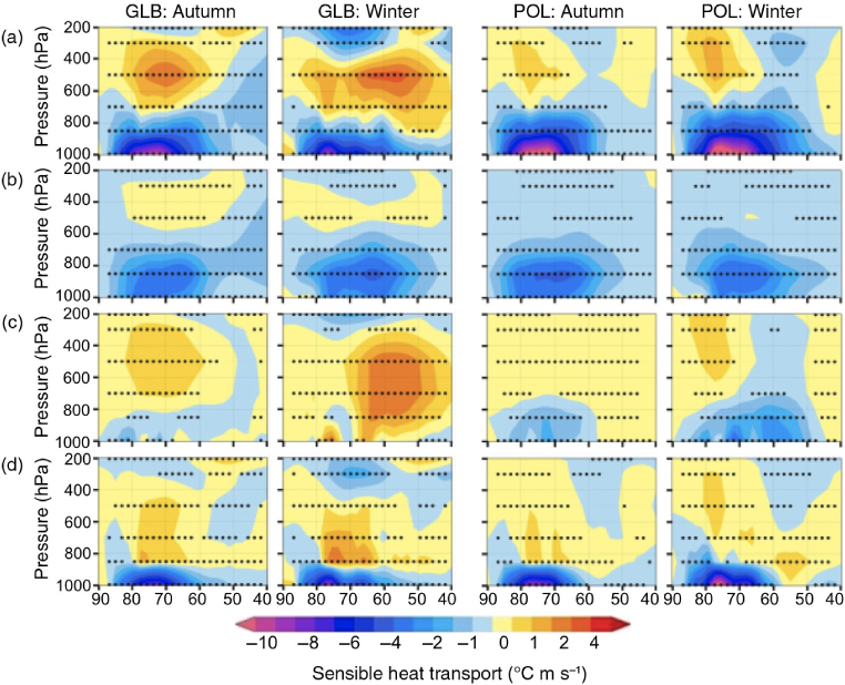
Fig. 3
Enhancement of northward heat transport. Change of zonally averaged meridional transport of sensible heat (°C·m·s−1) in autumn and winter from 40 to 90°N during the sea-ice-free period relative to control climate computed with global (GLB) and polar (POL) forcings. The total heat transport (a) is decomposed into transport by transient eddies (b), large-scale stationary eddies (c) and the mean meridional circulation (d). Northward transport is positive and southward is negative. Stippled areas represent statistically significant changes with confidence level 95%. Note that the colour scale is different than in Fig. 2.
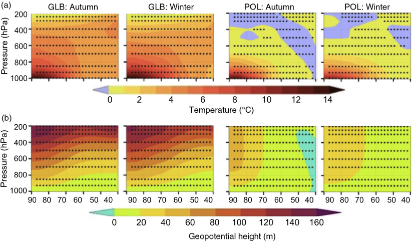
Fig. 4
Changes in the polar troposphere due to different climate forcings. Change of zonally averaged: (a) air temperature (°C) and (b) geopotential height (m) in autumn and winter from 40 to 90°N during the sea-ice-free period relative to control climate computed with global (GLB) and polar (POL) forcings. Stippled areas represent statistically significant changes with confidence level 95%.
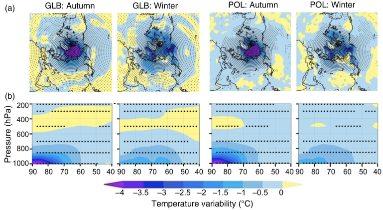
Fig. 5
Change of air temperature in the polar atmosphere. Change of subseasonal variability of: (a) near-surface air temperature (°C) and (b) seasonally averaged air temperature from 40 to 90°N. Both plots represent the sea-ice-free period relative to control climate in autumn and winter, computed with GLB and POL forcing. Stippled areas represent statistically significant changes with confidence level 95%.
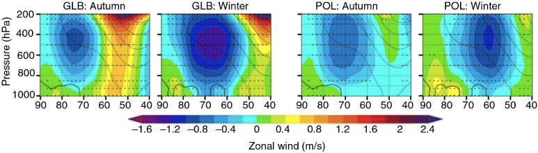
Fig. 6
Zonal-wind evolution. Change of zonally averaged zonal wind (m·s−1) in autumn and winter during the sea-ice-free period relative to control climate computed with global and polar forcings. Contours indicate the zonal wind (contour interval of 5 m·s−1, zero contour thickened) distributions from the control run. Stippled areas indicate statistically significant changes with confidence level 95%.
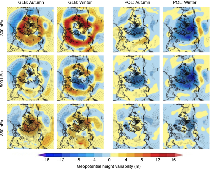
Fig. 7
Oscillation of planetary waves and climate forcing. Change of subseasonal GPH variability (m) at three levels of the troposphere in autumn and winter during the sea-ice-free period relative to control climate computed with global (GLB) and polar (POL) forcing. Stippled areas represent statistically significant changes with confidence level 95%.