
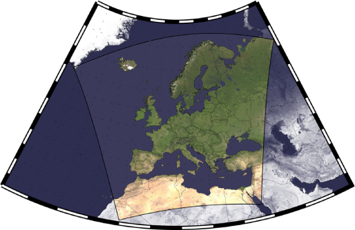
Fig. 1
CORDEX-EUR11 domain (colour-shaded area).
Table 1. Domain specification
Rotated North Pole−162.0, 39.25Lower left corner in rotated coordinates−23.375, −28.375Grid spacing0.11°Number of grid points424×412Number of vertical levels40Top of the model atmosphere22 700 m
Table 2. Observation stream for reanalysis
RadiosondesPILOTUpper-air windTEMPUpper-air wind, temperature,
humidityScreen-level wind,
humidity,
geopotentialAircraftAIREPWind, temperatureAMDARWind, temperatureACARSWind, temperatureWind profilerUpper-air windSurface systemsSYNOPSurface pressure,
wind, humiditySHIPSurface pressure,
wind, humidityDRIBUSurface pressure,
wind, humidity
{ label needed for table-wrap[@id='T0003'] }
Table 3. Observation error standard deviations for sea observing systems
DRIBUU/V [m/s]5.4DRIBUΦ [m]14.0SHIPΦ [m]14.0
{ label needed for table-wrap[@id='T0004'] }
Table 4. Observation error standard deviations for upper-air and surface systems
10002.04.31.20.091.22.57.03.68502.44.41.00.131.02.58.03.67002.55.20.70.120.73.08.65.85003.48.40.40.130.53.512.16.84003.59.80.40.130.54.03003.710.70.50.140.64.02503.511.80.50.140.64.02003.513.20.60.140.74.01503.415.20.70.140.84.01003.318.10.80.140.94.0703.219.50.80.141.04.0503.222.50.90.141.14.0303.325.00.90.141.14.0203.632.01.00.141.24.0104.540.01.20.141.44.0
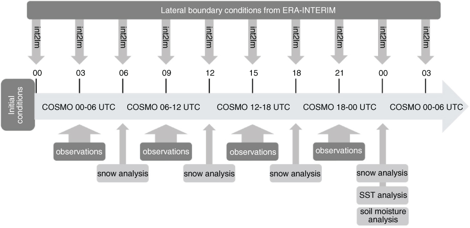
Fig. 2
Process cycle of the ensemble nudging reanalysis system for one exemplary ensemble member. The cycle is repeated for all members in parallel. All members are provided with the same lateral boundary conditions. The tool int2lm interpolates the fields from the steering model to the COSMO grid.
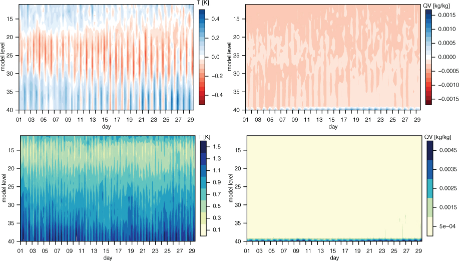
Fig. 3
Analysis increments for June 2011. The upper panels show spatially averaged analysis increments in dependency of model level and time of day for temperature (left) and specific humidity (right). The analysis increments are aggregated over 6-hourly analysis cycles from 00, 06, 12 and 18 UTC. Model levels 20 and 30 are located at about 550 hPa and 100 hPa above the surface, respectively. For temperature red colour indicates a too warm model and blue colour indicates a too cold model. For specific humidity red colour means that the model is too moist while blue colour means that it is too dry. The lower panels show the horizontal variability in terms of standard deviations of analysis increments for temperature (left) and specific humidity (right) in dependency of model level and time of day.
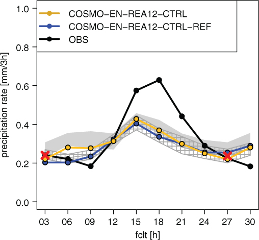
Fig. 4
Diurnal cycle of 3-hourly precipitation rates in ensemble of reforecasts of COSMO-EN-REA12, initialised at 00 UTC (shown as hatched area, 5 % to 95 % percentiles, control run blue points), reanalysis ensemble (shown as shaded area, 5 % to 95 % percentiles, control run yellow points) and corresponding rain gauge observations (black dots). Shown for German stations, see Fig. 8. The red crosses mark the median of the reforecast ensemble at 03 and 27 hours lead time.
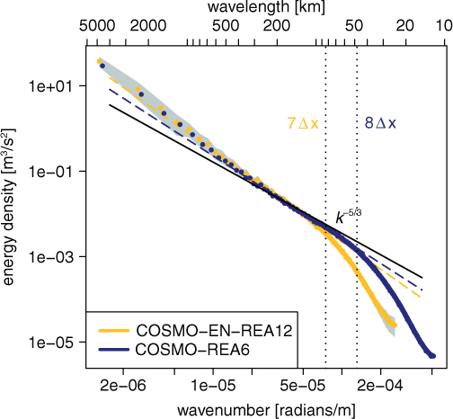
Fig. 5
Horizontal kinetic energy spectra for COSMO-EN-REA12 (yellow points) and COSMO-REA6 (blue points) in dependence of wavelength and wave number. The grey area shows the uncertainty estimated from the ensemble. The vertical lines mark the effective resolution of the reanalysis systems. The continuous line shows k −5/3 line. The dashed yellow and blue lines show slopes of spectra at the mesoscale, both of which are slightly steeper than k −5/3.
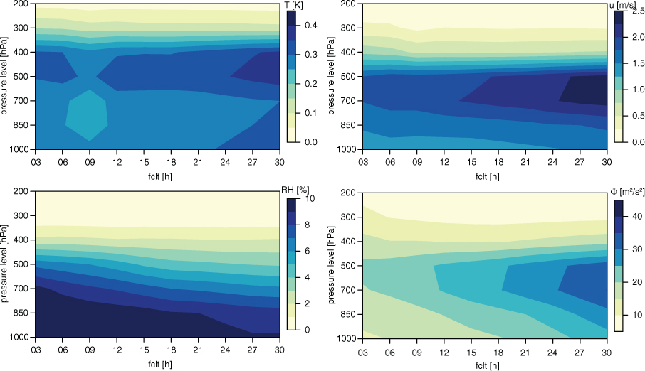
Fig. 6
Monthly mean evolution of horizontally averaged spread (over German subdomain) as a function of pressure levels and forecast lead time. Data are from reforecasts initialised at 00 UTC for experiment for June 2011. Upper panels are for temperature (left) and zonal wind (right), lower panels for relative humidity (left) and geopotential (right).
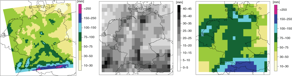
Fig. 7
Monthly precipitation climatologies for Germany for June 2011 based on ensemble mean of COSMO-EN-REA12 (left) and ERA-Interim (right). In the middle, the uncertainty (spread) of the monthly integrated precipitation estimated by COSMO-EN-REA12 is shown.
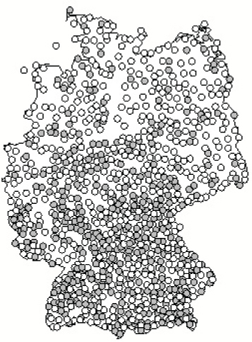
Fig. 8
Rain gauges used for verification. The grey stations are used for the probabilistic verification, and the white ones are additionally used for the deterministic verification.
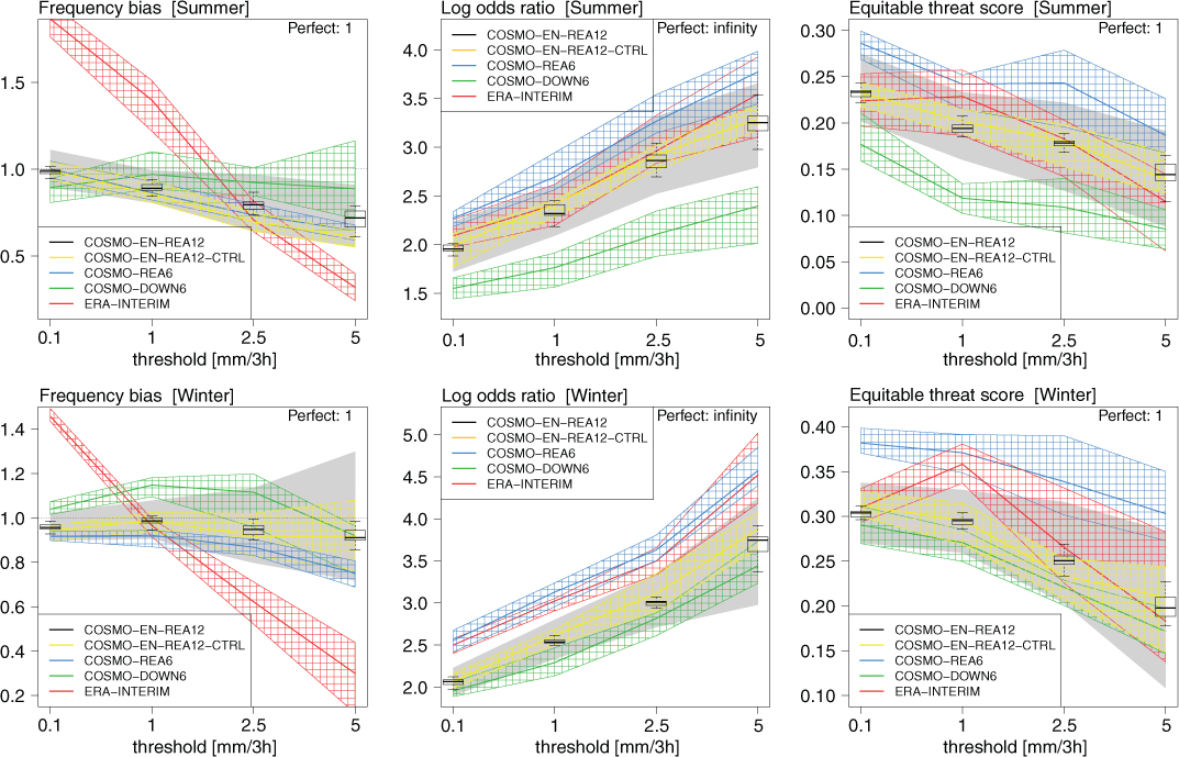
Fig. 9
Verification measures (from left to right: frequency bias, log odds ratio, equitable threat score) based on the (2×2) contingency table for binary events as a function of threshold for 3-hourly accumulated precipitation. The upper panels show the summer experiment (June 2011), and the lower ones show the winter experiment (December 2011). The control run of the ensemble nudging experiments is depicted in yellow and the nudging ensemble as boxplots. ERA-Interim is presented in red, COSMO-REA6 in blue and COSMO-DOWN6 in green. The solid lines represent the median of 1000 bootstrap samples while the hatched areas are 95 % confidence intervals. For each of the ensemble members, 1000 bootstrap samples have been drawn. The grey shaded area presents the 95 % confidence interval of the resulting 20 000 bootstrap samples of the ensemble members.
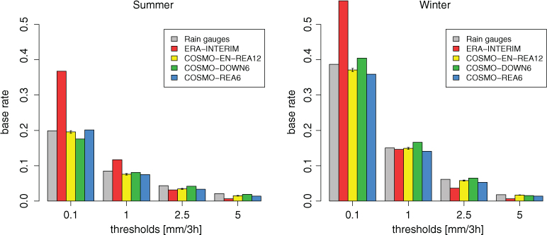
Fig. 10
Base rates of threshold exceedance for 3-hourly accumulated precipitation in the summer and winter experiments. Sample size approximately 255 000.

Fig. 11
Analysis rank histograms for 6-hourly accumulated precipitation in the summer experiment (left panel) and the winter experiment (right panel) with the probabilistic regional reanalysis system.
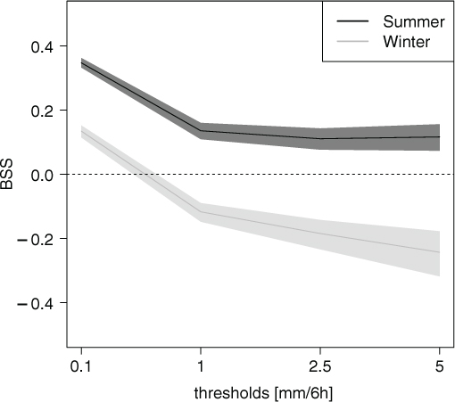
Fig. 12
Brier skill score of ensemble nudging versus ECMWF-EPS for 6-hourly accumulated precipitation. The summer experiment is illustrated in dark grey and the winter experiment in light grey. The solid lines represent the medians and the shading represents the sampling uncertainty as given by the 95 % quantile of 1000 bootstrap samples.
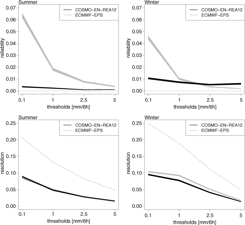
Fig. 13
Decomposition of the Brier score: 5 % to 95 % quantiles of 1000 bootstrap samples of reliability (upper panels) and resolution (lower panels) for the summer (left) and winter (right) experiments. The thin dotted lines indicate the maximally achievable resolution if the reliability was perfect.
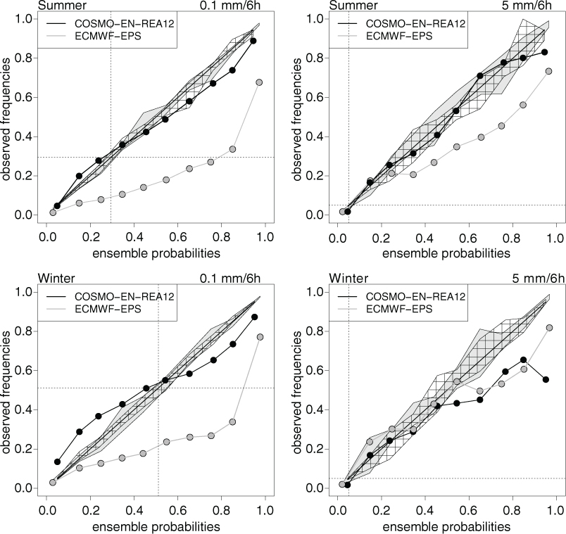
Fig. 14
Reliability diagrams for 0.1 mm/6 h (left panels) and 5 mm/6 h (right panels) decision thresholds for the summer and winter experiments. The grey shaded area represents consistency intervals for the ECMWF-EPS and the black hatched one for ensemble nudging. These represent the areas within which the ensemble is reliable. The dashed vertical and horizontal lines represent the climatological observed frequency of the events.
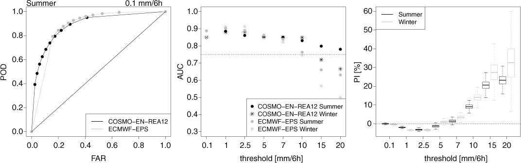
Fig. 15
ROC curve measures. The left panel shows exemplary ROC curves for 0.1 mm. The panel in the middle shows absolute values for the area under the ROC curve (AUC) for different thresholds. In both panels, COSMO-EN-REA12 is depicted in black and the ECMWF-EPS in grey. The right panel depicts the percentage improvement (PI) in terms of AUC of ensemble nudging over the ECMWF-EPS for the summer (black boxplots) and winter experiments (grey boxplots).