
Fig. 1
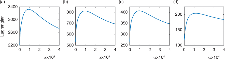
Lagrangian versus the smoothing parameter α calculated using eq. (31), based on the leading smooth EOF of the extratropical NH SLP anomalies for 2.5°×2.5° (a), 5°×5° (b), 5°×10° (c) and 10°×10° (d) latitude–longitude grid.
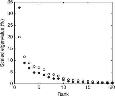
Fig. 2
Eigenvalues µ of the generalised eigenvalue problem [eq. (21)] for the winter SLP anomalies over the Northern Hemisphere for the smoothed problem (filled circle) and the non-smoothed (α=0) problem (open circle). The eigenvalues are scaled by the total variance of the SLP anomalies and transformed to a percentage, so, for example, the spectra given by the open circles provide the percentage of explained variance of the EOFs.
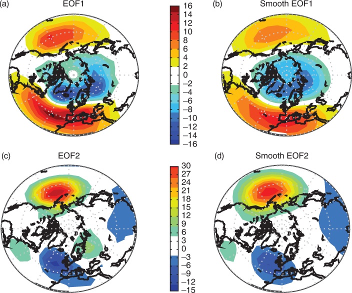
Fig. 3
Leading two EOFs (a, c) and regularised EOFs (b, d) of the Northern Hemisphere SLP anomalies based on the 10°×10° latitude–longitude grid. The smoothing is based on the optimal value of the Lagrangian (Fig. 1d).
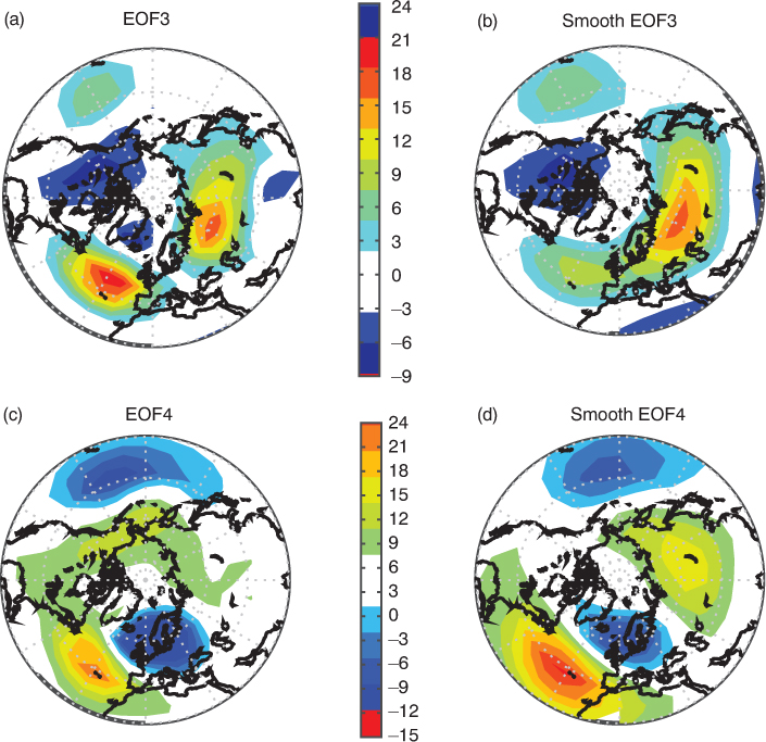
Fig. 4
As in Fig. 3 but for the third and fourth EOFs (a, c) and smooth EOFs (b, d) patterns.
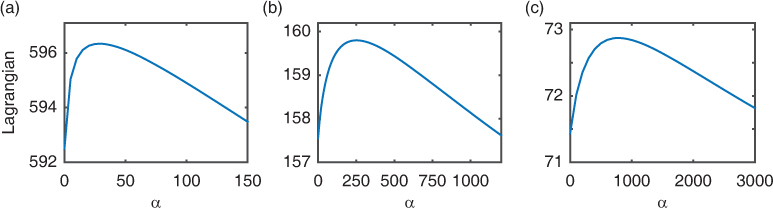
Fig. 5
As in Fig. 1 but for the SLP anomalies over the tropical region for 2.5° (a), 5° (b) and 7.5° (c) latitude–longitude grid.
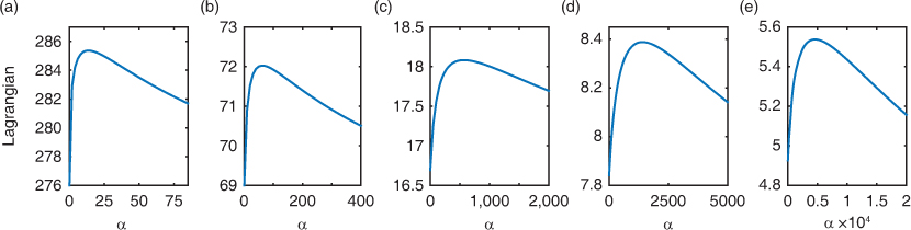
Fig. 6
As in Fig. 1 but for the SST anomalies based on the 2° (a), 4° (b), 8° (c), 12° (d) and 16° (e) latitude–longitude grids.
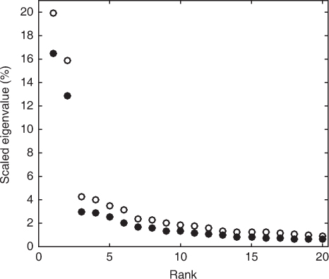
Fig. 7
As in Fig. 2 but for the SST anomalies at 16° latitude–longitude resolution grid.
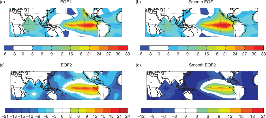
Fig. 8
Leading two EOFs (a, c) and smooth EOFs (b, d) of the SST anomalies using the 16°×16° latitude–longitude grid. The smoothing is based on the optimal value of the Lagrangian (Fig. 6e).
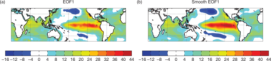
Fig. 9
Leading EOF (a) and smooth EOF (b) of the SST anomalies using the 2°×2° latitude–longitude grid and the optimal smoothing parameter (Fig. 6a).
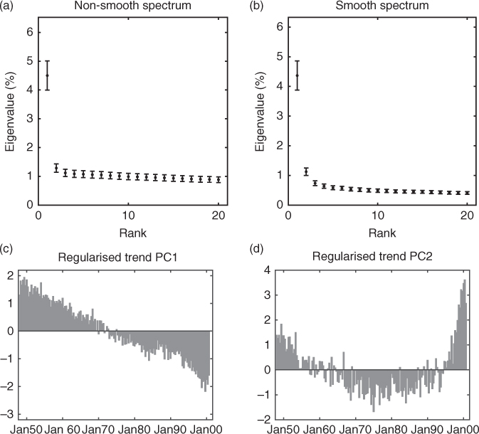
Fig. 10
Eigenspectrum, given in terms of percentage of explained variance, of the covariance (or correlation) matrix of the inverse ranks of the SLP anomalies with a reduced resolution of 5°×5° grid for the non-regularised (a) and regularised (b) cases, along with the regularised first (c) and second (d) trend PCs associated with the leading two eigenvalues shown in (b). The optimal smoothing parameter, α=60, is used in (b).
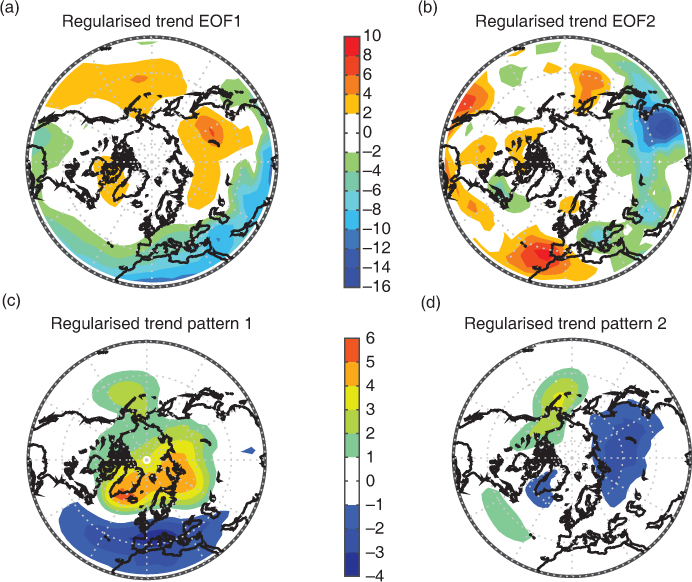
Fig. 11
The leading two regularised trend EOFs (a, b) of the SLP anomalies, corresponding to the leading two eigenvalues of Fig. 10b, and the associated trend patterns (c, d) obtained by projecting the SLP anomalies onto the trend EOFs and then regressing back onto the same anomalies. Contour interval in (c, d) is 1 hPa.