
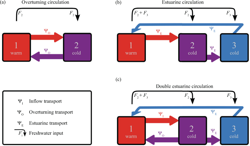
Fig. 1
Three-box model configurations. (a) Overturning (negative estuarine) circulation with volume transport ΨO, identical to the configuration of Stommel (1961), (Section 2.1); F 2 indicates the freshwater input into basin 2. (b) Estuarine circulation with volume transport ΨE, identical to the configuration of Rooth (1982), (Section 2.2). F 2 and F 3 indicate the freshwater input into the double estuary (basins 2 and 3). (c) Double estuarine circulation combining an overturning and estuarine branch (Section 3). The inflow transport ΨI into the double estuary is the sum of the overturning and estuarine transports. Arrows depict positive transports by convention.
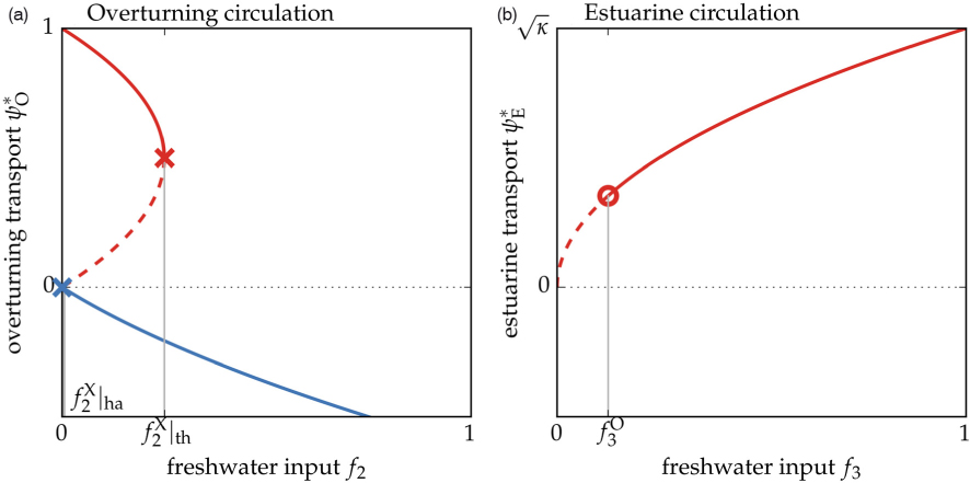
Fig. 2
Bifurcation diagrams for Stommel and Rooth's models. (a) Equilibrium overturning transport as a function of freshwater input into basin 2. Red and blue curves indicate thermal and haline regimes, respectively. X's indicate saddle-node bifurcations [cf. eqns. (11) and (12)]. (b) Equilibrium estuarine transport as a function of freshwater input into basin 3. O indicates a Hopf bifurcation [cf. eqns. (22)]. In both panels, solid (dashed) lines indicate stable (unstable) equilibria.
Table 1. Model parameters
Present state observations Salinity contrast Atlantic inflow and overflowsΔS120.3 psu Salinity contrast overflows and polar waterΔS230.9 psu Temperature contrast Atlantic inflow and outflowsΔT8 K Volume transport Atlantic inflowΨI8.5 Sv Volume transport overflowsΨO6 SvParameters Thermal expansion coefficientα10−4 K−1 Haline contraction coefficientβ8×10⁻⁴ psu−1 Hydraulic constant overturning branchkO104 Sv Hydraulic constant estuarine branchkE3×103 Sv Volume basin 2V21016 m3Scaling terms Timet40 yr Freshwater input (relative to 35 psu)F i 230 mSv Salinity contrastΔS ij 1 psu Volume transportΨ8 Sv
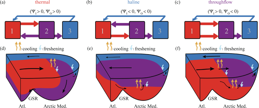
Fig. 3
Three flow regimes of the double estuary. (a–c) Qualitative flow directions which define the different regimes. (d–f) An interpretation of the corresponding regimes in an Arctic Mediterranean setting. The present state of the Arctic Mediterranean can be characterised as a thermal circulation (panel d).
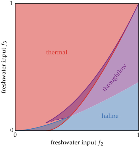
Fig. 4
Phase-space diagram for the double estuarine circulation. Colour shading indicates which circulation regime(s) can be stable as a function of both freshwater parameters f 2 and f 3. So-called bistability occurs where two regimes overlap. Solid lines indicate saddle-node bifurcations [cf. eqns. (32–34)]; the dashed line indicates a Hopf bifurcation [eq. (22)]. The diagram is drawn for the symmetrical case κ=1 and V 1=V 2=V 3.
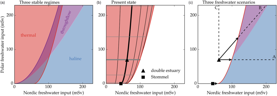
Fig. 5
Phase-space diagram for the Arctic Mediterranean. (a) As in Fig. 4, scaled as described in Section 4. (b) Stable region of the thermal regime. Contours, interval 1 Sv, indicate constant overturning (black) and estuarine transport (grey). Thick lines correspond to observed transports (cf. Table 1). Markers indicate the ‘present state’ in the double estuary model and in Stommel's model. (c) From the ‘present state’, three dashed lines indicate scenarios for increased freshwater input in the double estuary model. Arrows indicate the required freshwater increase along each scenario to induce an abrupt transition into either the throughflow or haline regime. An additional scenario is indicated for Stommel's model for increased Nordic freshwater input.
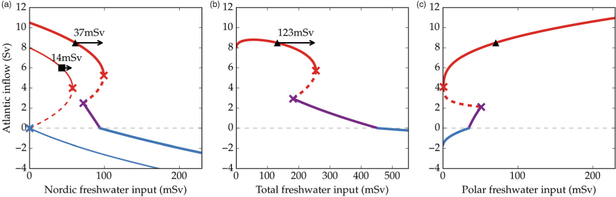
Fig. 6
Bifurcation diagram for three scenarios of increased freshwater input into the Arctic Mediterranean. Equilibrium solutions for ΨI * are shown along the trajectories A, B and C indicated in Fig. 5c. As a reference, the bifurcation diagram of the overturning (Stommel, Fig. 2a) is shown in the left panel. ‘Present state’ (triangle and square) is defined in Fig. 5b. Arrows are equivalent to those in Fig. 5b, indicating the required freshwater increase to destabilise the thermal circulation and induce an abrupt transition. The three Scenarios A, B and C are described in detail in the text.