
Table 1. Experiments used in this study
ControlECMWF operational configuration (cycle 38r2) with all observations but with T511 horizontal resolution.PerturbationScientifically identical to the control, but with a technical modification that results in numerical differences in some operators in the data assimilation, compared to the control. See Section 4.AMSU-A denialThe AMSU-A on Metop-A has been removed from the observing system.
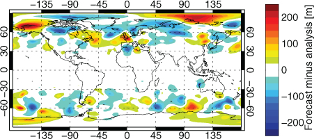
Fig. 1
Day-5 forecast minus analysed geopotential height at 500 hPa in the control experiment, at 00Z on 31 January 2012.
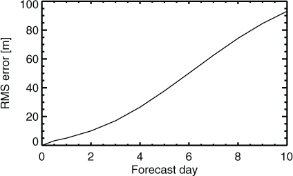
Fig. 2
RMS error of NH geopotential height at 500 hPa in the control experiment, as a function of forecast lead time, for the control experiment, aggregated over 1 January 2011 to 31 July 2013.
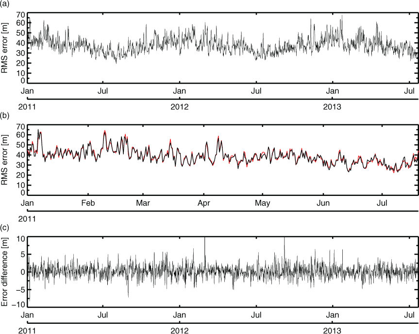
Fig. 3
Time series of (a) RMS error of 500-hPa NH geopotential height at day 5 in the control experiment (black), verified against an own-analysis reference. (b) As (a), but covering a shorter period of time and including scores from the AMSU-A experiment (red). (c) Experiment minus control over the full time period.
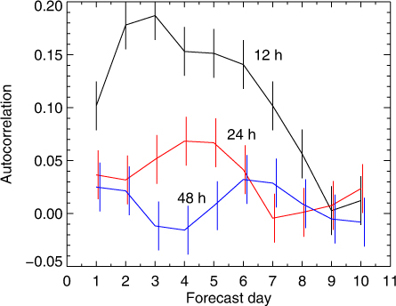
Fig. 4
Time autocorrelation of paired differences (AMSU-A Denial minus control) in RMS error of NH geopotential height at 500 hPa, as a function of forecast lead-time. Autocorrelations are shown for forecasts separated by 12 h (black), 24 h (red) and 48 h (blue). This pattern is representative of all tropospheric levels in the NH and for other choices of forecast score, such as anomaly correlation, or the RMS error in temperature or vector wind. However, autocorrelation becomes very significant in the stratosphere, where systematic errors dominate RMS forecast scores, and it is slightly larger in the SH. Error bars have been estimated with a Monte-Carlo approach: they are represented by the standard deviation of a large number of lag-1 autocorrelations estimated from samples of 1885 normally distributed random numbers.
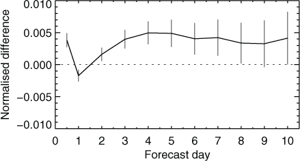
Fig. 5
Normalised change in RMS error of NH geopotential height at 500 hPa (AMSU-A denial minus control) as a function of forecast lead-time, aggregated over 1866–1885 forecasts between 1 January 2011 and 31 July 2013. Vertical bars (which should not be confused with regular error bars) give the 95 % confidence range.
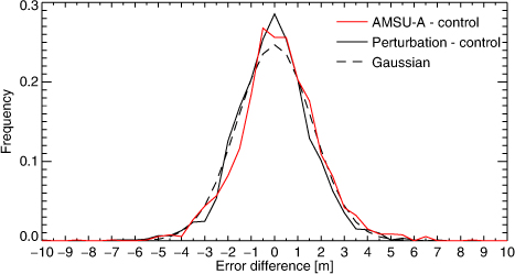
Fig. 6
Histograms of paired differences in NH RMS 500-hPa geopotential height errors at day 5. A Gaussian is plotted that has the same standard deviation as the perturbation minus control population. The integral of this histogram is normalised to 1 (it is a PDF). Bins are 0.5 m in size. Each population has 1876 members.
Table 2. Statistical properties of the paired differences in NH RMS 500-hPa geopotential height errors at various forecast ranges
AMSU-A-30.070.55−0.102.67 control50.181.770.473.6070.263.900.211.92100.388.43−0.061.27Perturbation-3−0.010.48−0.131.76 control5−0.041.62−0.121.6170.123.630.141.10100.358.300.080.51
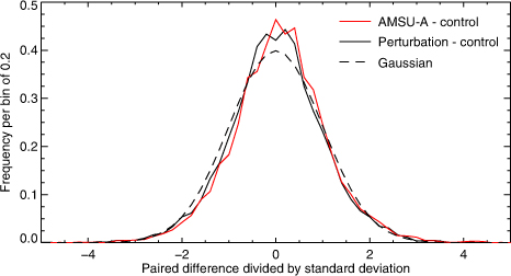
Fig. 7
Histograms of paired differences in RMS 500-hPa geopotential height errors, standardised by dividing by the standard deviation of four sub-populations (day 4 and day 10 in both SH and NH). This gives a population of 7464 in each histogram. The dashed line is the standard Gaussian. Bin size is 0.2 and the integral of the PDF across all bins is 1.
Table 3. Skewness, kurtosis and chi-squared of the populations shown in Fig. 7
AMSU-A- control0.1451.391045Perturbation- control−0.0531.30168.9
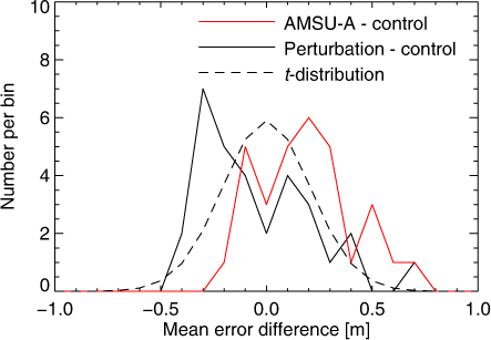
Fig. 8
The uncertainty of forecast differences computed over one month (i.e. 60 forecasts). The figure shows histograms of the mean of paired differences in NH RMS 500-hPa geopotential height errors at day 5. There are 31 different contiguous 60-forecast samples available in the 2.5-yr experimental period. Bin size is 0.1 m. The dashed line shows the t-distribution transformed into the space in which we are computing means.
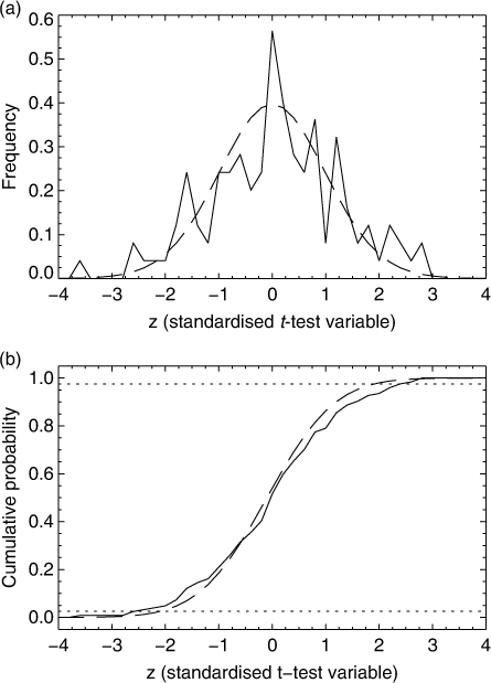
Fig. 9
The result of performing t-tests on samples from the explicitly generated null population, that is, the differences between the perturbation and control experiments: (a) PDF of z-tests generated from blocks of 60 paired forecast differences (solid) and the Student's t-distribution (dashed); (b) CDF of the same. Dotted horizontal lines indicates the 2.5 and 97.5 % quantiles, the limits of the 95 % confidence test. Based on a total of 124 independent blocks, 31 from each of the SH and NH at day 4 and day 10. Bin size is 0.25.
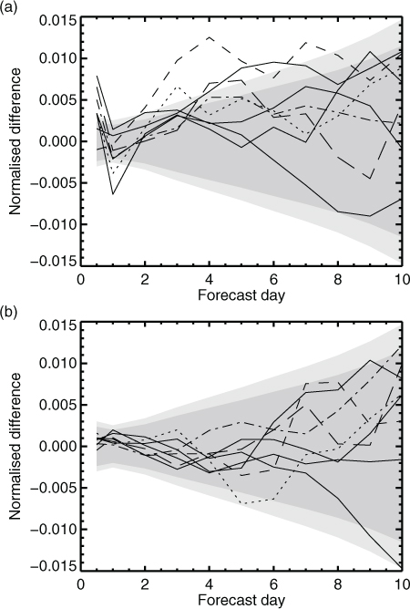
Fig. 10
Normalised change in NH 500-hPa height RMS forecast error: a) AMSU-A minus control; b) perturbation minus control. Separate lines are shown for eight independent blocks of 230 forecasts. Change in error is normalised by the RMS error of the control experiment. The shading indicates the 95 % confidence range estimated in the normal way (no inflation, dark grey) or with the 25 % inflation factor estimated from the explicit null population (light grey). To compute the confidence range, the standard deviation of paired differences computed from all 2.5 yr of samples in the null distribution has been used. It is centred on zero, which is more statistically correct than centring on the experimental result (the method used in Fig. 5). This approach gives less visual clutter when many experiments are presented on the same figure.
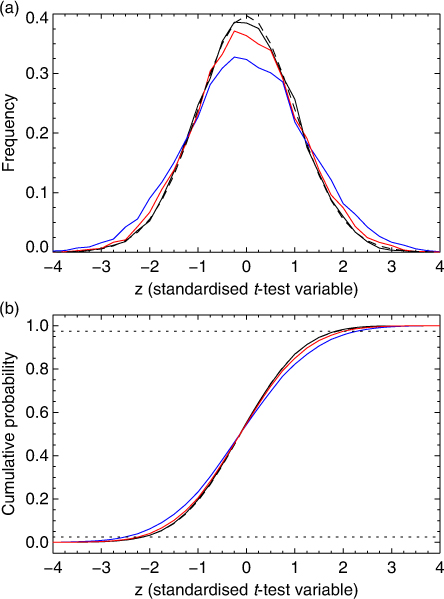
Fig. 11
As Fig. 9, but based on randomly generated populations representing a true Gaussian (dashed), an uncorrelated non-Gaussian population with a kurtosis of 1.3 (solid black, barely distinguishable from the Gaussian), a Gaussian population with 0.07 autocorrelation, representing forecasts made 24 h apart (red) or with [0.15, 0.07] autocorrelation, representing forecasts made 12 h apart (blue). Results are based on 16 666 non-overlapping blocks each containing 60 samples.
Table 4. Estimates of k using autoregressive models and the autocorrelations for day-5 NH geopotential paired differences from Fig. 4, either for 12 or 24 h separation between forecasts
ModelForecast separationLag-1Lag-2k
AR(1)240.07N/A1.07±0.02AR(1)120.15N/A1.16±0.02AR(2)120.150.071.22±0.04
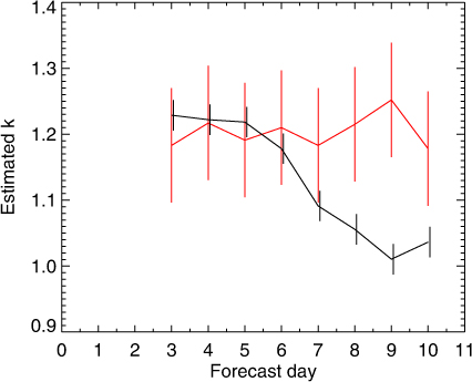
Fig. 12
Estimates of the inflation factor k for forecasts separated by 12 h made using the AR(2) technique with autocorrelations from Fig. 4 (black) or using the non-parametric technique applied to blocks of 30 paired differences from the explicit null population (red).
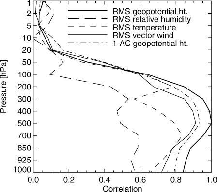
Fig. 13
Correlation of paired differences in NH day-5 RMS 500-hPa geopotential height error with paired differences in other measures of forecast error on the same forecast day for the same hemisphere. Anomaly correlation of geopotential height error (AC) has been transformed to (1-AC) to give positive rather than negative correlation.
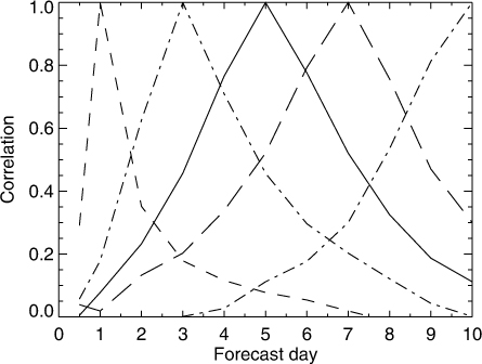
Fig. 14
Correlation of paired differences in NH RMS 500-hPa geopotential height error across forecast day, for forecasts with the same base time. Examples shown for day 1, day 3, day 5, day 7 and day 10.
Table 5. The probability of a particular number of false results (type-I errors) being generated by N significance tests computed using a 95 % confidence range
N=40.810.170.010.000.000.000.000.00N=80.660.280.050.010.000.000.000.00N=120.540.340.100.020.000.000.000.00N=160.440.370.150.040.010.000.000.00N=320.190.330.270.140.050.020.000.00N=1240.000.010.040.080.120.160.160.15
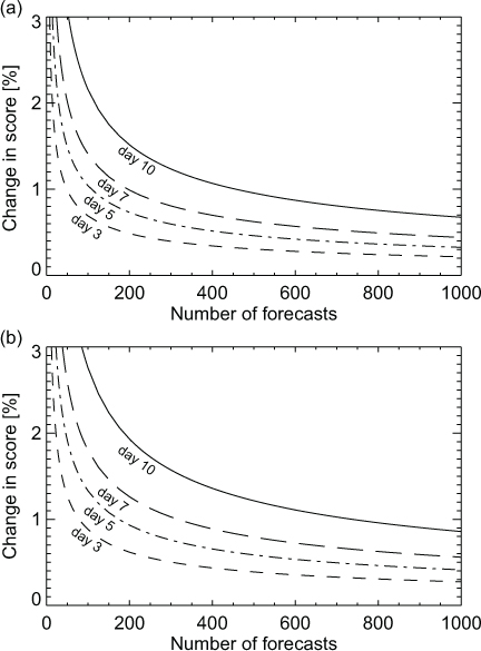
Fig. 15
95 % confidence range for 500-hPa geopotential height in the NH, expressed as a percentage of the RMS error of the control, and as a function of the number of forecasts in the sample used to compute the scores: (a) without correction for multiplicity; (b) with an N=4 Šidák correction for multiplicity. If d 95 is the range read from this figure, the full confidence range is ±d 95.
Table 6. In order to give statistically significant results at 95% confidence range for a certain change in the NH 500-hPa geopotential height forecast sores at day 5, the top section shows the number of samples required, and the bottom section the number of days of experimentation required
Number of samples required
Forecasts every 12 h (k=1.22)291084241690Forecasts every 24 h (k=1.07)23843271301Forecasts every 48 h (k=1)20732861136Days of experimentation
Forecasts every 12 h (k=1.22)1454212845Forecasts every 24 h (k=1.07)20843271301Forecasts every 48 h (k=1)401465722272
Table 7. Sampling uncertainty of inflation factors k generated from autocorrelation parameters r 1 and r 2, which themselves have been estimated from a sample of finite size
Statistics of inflation factors generated from forecasts every 12 h (simulated by [0.025, 0.065, 0.82, 0.065, 0.025] convolution)
100.8690.3240.222.14601.1610.2190.651.983601.2140.0900.961.5918851.2230.0381.111.35Statistics of inflation factors generated from forecasts every 24 h (simulated by [0.035, 0.93, 0.035] convolution)
100.8110.3050.212.02601.0250.1900.561.773601.0650.0770.851.3718851.0710.0330.981.17
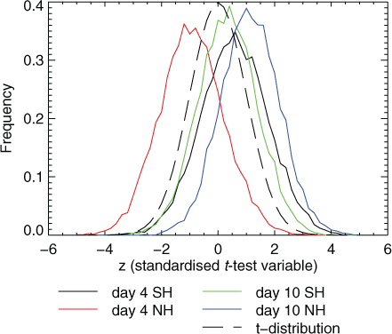
Fig. 16
(a) PDF of z-tests generated from bootstrapped samples of 720 forecasts (solid) and the Student's t-distribution (dashed). Based on a total 10 000 for each of the four independent populations.