
Fig. 1
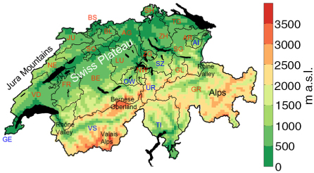
WRF terrain height of the innermost model domain in m a.s.l. (colour scheme; horizontal grid size of 3 km). Places mentioned in the text, main regions of Switzerland (i.e. Jura Mountains, Swiss Plateau, and Alps), lakes, and cantonal boundaries are indicated. Two-letter abbreviations of the GUSTAVO cantons are given in blue letters [Geneva (GE), Uri (UR), Schwyz (SZ), Ticino (TI), Appenzell-Innerrhoden (AI), Valais (VS), Obwalden (OW)] and of the remaining cantons in red letters [non-GUSTAVO cantons; Aargau (AG), Appenzell-Ausserrhoden (AR), Bern (BE), Basel-Country (BL), Basel-City (BS), Fribourg (FR), Glarus (GL), Grisons (GR), Jura (JU), Lucerne (LU), Neuchâtel (NE), Nidwalden (NW), St. Gallen (SG), Schaffhausen (SH), Solothurn (SO), Thurgau (TG), Vaud (VD), Zug (ZG), Zurich (ZH)].
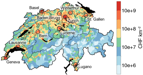
Fig. 2
Assets in CHF per km2 at municipal level for year-2009 asset distribution (colour scheme; base 10 logarithmic scale) as prescribed in the climada model (i.e. number of inhabitants in 2009 multiplied by 250 000 CHF). Circles indicate the 10 major agglomerations of Switzerland on 1 January 2009 (according to the Swiss Federal Statistical Office). Cantonal boundaries and lakes are outlined.
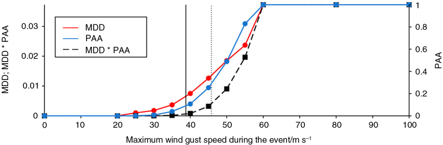
Fig. 3
Mean damage degree (red; left y-axis), percentage of assets affected (blue; right y-axis), and product of MDD and PAA (black; left y-axis) as a function of maximum wind gust speed during the windstorm event. A linear interpolation was applied between two consecutive points (denoted with a straight line segment). The maximum downscaled surface wind gust speed over Switzerland during ‘Lothar’ (added with 7 m s−1; i.e. the average bias of estimated surface wind gust speeds using the WPD method compared to instrumental wind gust speed measurements in case of ‘Lothar’; see Table 1) is marked by the solid (dotted) vertical line.

Fig. 4
(a) 20CR ensemble mean surface wind speed in m s−1 (2° by 2° latitude–longitude grid) at the time of windstorm ‘Lothar’ on 26 December 1999, 12 UTC. The red box indicates domain 1 (25°N–66°N, 34°W–49°E) of the applied stepwise dynamical downscaling of the 20CR ensemble mean using WRF. (b–d) Analogous to (a), but shown are the downscaled surface wind speeds in m s−1 for downscaling domain 1, domain 2 (43 °N–53°N, 1°E–14 °E), and domain 3 (46°N–48°N, 6°E–11°E); grid sizes of 45 km, 9 km, and 3 km. The border of Switzerland and Swiss lakes are marked. The grey contours in (d) show the 1500 m a.s.l. WRF terrain height.
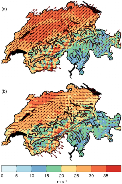
Fig. 5
Wind gust footprints for (a) ‘Lothar’ and (b) ‘Joachim’ in m s−1 (colour scheme). Vectors indicate both direction and magnitude of the surface wind at the times when wind gust speeds were maximal in Switzerland. The WRF terrain height 1500 m a.s.l. contour line and lakes are outlined.
Table 1. Average bias of estimated surface wind gust speeds using the WPD method (COS method) compared to instrumental wind gust speed measurements from the SMN dataset in m s−1 (i.e. estimated wind gusts minus measured gusts) for windstorms ‘Lothar’ and ‘Joachim’
Windstorm eventWind gust estimationMountain stationsStations in valleysStations in flat terrainAll stations
‘Lothar’WPD−17.0−2.5−5.8−7.0COS−18.4−6.0−7.6−9.3‘Joachim’WPD−5.43.70.20.2COS−4.22.5−0.2−0.1

Fig. 6
(a) Simulated loss per km2 at municipal level for ‘Lothar’ under year-2009 asset distribution. (b, c) Insured loss per km2 for ‘Lothar’: (b) the sum of MOB movable property and building loss data at postal code level and (c) building loss data at cantonal level provided by the IRV. MOB is not allowed to insure damage to movable properties and buildings in the cantons of Vaud and Nidwalden [marked grey in (b)]. Grey cantons in (c) are not covered by the IRV (GUSTAVO cantons), no damage information is available for the canton of Neuchâtel (white), and the cantons with the highest losses per km2 are marked because loss maxima are not discernible. Note that the same colour scheme (base 10 logarithmic scale) was used for simulated losses as well as insured losses in this study. The loss data were classified into loss categories (ranging from low to high losses) because the insurance loss data are proprietary. Cantonal boundaries and lakes are outlined.
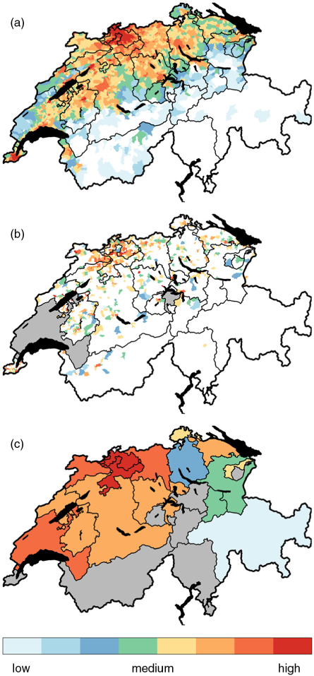
Fig. 7
The same as Fig. 6, but for windstorm ‘Joachim’.
Table 2. Ratio of MOB insured losses to losses simulated based on MOB insurance portfolios at postal code level (here, distinction made between movable properties and buildings) for ‘Lothar’ and ‘Joachim’
‘Lothar’WPD13.759.4COS8.922.6COSMO/COS1.11.4‘Joachim’WPD1.62.9COS0.20.3COSMO/COS0.50.6
[i] Loss simulations were performed on the basis of wind gust estimates from the operational versions of the MeteoSwiss COSMO model using the COS wind gust estimation method (COSMO/COS) as well as from dynamical downscaling of the 20CR ensemble mean using WRF and applying the WPD and COS wind gust estimation methods.
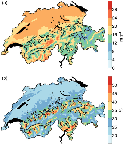
Fig. 8
(a) Composite mean of the wind gust footprints for all 84 windstorm events in m s−1 (colour scheme). (b) Composite coefficient of variation in %; the composite coefficient of variation was calculated from the ratio of the composite standard deviation to the composite mean. The WRF terrain height 1500 m a.s.l. contour line and lakes are outlined.
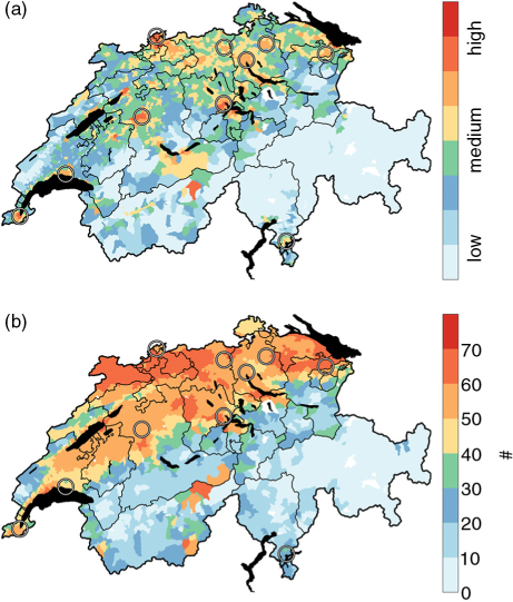
Fig. 9
(a) Composite mean of simulated loss per km2 at municipal level for all 84 windstorm events (colour scheme; base 10 logarithmic scale). (b) For each municipality, number of windstorm events with simulated loss greater than zero (maximum number = 84 events). Circles indicate the 10 major agglomerations of Switzerland in 2009. Cantonal boundaries and lakes are outlined.
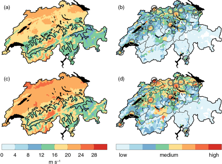
Fig. 10
(a, c) Composite mean of the wind gust footprints for the windstorm events in (a) 1871–1949 (43 events) and (c) 1950–2011 (41 events) in m s−1 (colour scheme). The WRF terrain height 1500 m a.s.l. contour line and lakes are outlined. (b, d) Composite mean of simulated loss per km2 at municipal level for the windstorm events in (b) 1871–1949 and (d) 1950–2011 (colour scheme; base 10 logarithmic scale). Circles indicate the 10 major agglomerations of Switzerland in 2009. Cantonal boundaries and lakes are marked.

Fig. 11
Simulated loss summed over all Swiss municipalities in CHF for all 84 windstorm events under year-2009 asset distribution (blue bars; base 10 logarithmic scale; see also Supplementary Table A1). The top 10 windstorm events are marked with red circles (Table 3).
Table 3. The top 10 windstorm events in Switzerland during the winter months October through March of 1871–2011 concerning simulated loss summed over all Swiss municipalities
11999-12-26100.0‘Lothar’21990-02-2751.9‘Vivian’31958-01-0749.9–41984-11-2346.1–51982-11-0844.3‘Once-in-a-century’ foehn storm62002-11-1535.8‘Uschi’71911-12-2234.1–82011-12-1733.8‘Joachim’91967-02-2331.9‘Adolph-Bermpohl’ windstorm101900-02-1420.9–
[i] Given is the date of the maximum downscaled surface wind gust speed over Switzerland during the respective event and the simulated loss for each event summed over all Swiss municipalities; expressed as a percentage of the simulated loss associated with ‘Lothar’ on 26 December 1999 (rank 1). If available/known, the name of the windstorm (associated low-pressure system) is given.
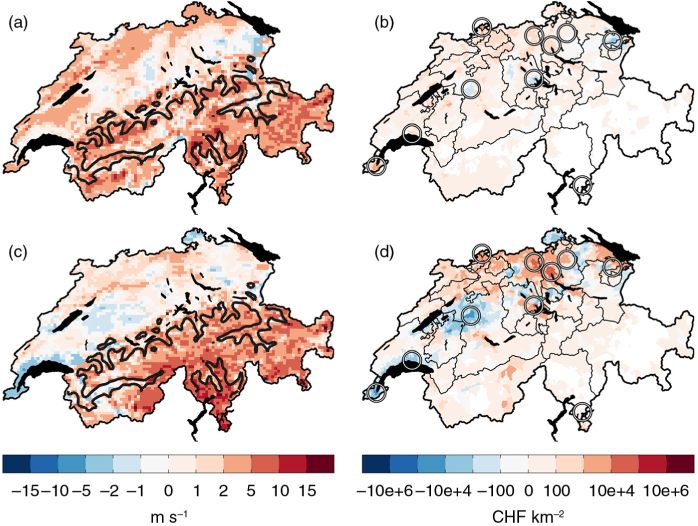
Fig. 12
The wind gust footprints for (a) the windstorm in February 1935 and (c) ‘Lothar’ were calculated first, based on (i) the ensemble mean approach and (ii) the ensemble maximum approach (see text for explanations), and the difference (ii) – (i) was computed subsequently (in m s−1; non-linear colour scheme). The WRF terrain height 1500 m a.s.l. contour line and lakes are outlined. (b, d) Analogous to (a, c), but shown are the differences between the corresponding simulated losses in CHF per km2 at municipal level under year-2009 asset distribution for the two approaches (colour scheme; base 10 logarithmic scale). Circles indicate the 10 major agglomerations of Switzerland in 2009. Cantonal boundaries and lakes are outlined.
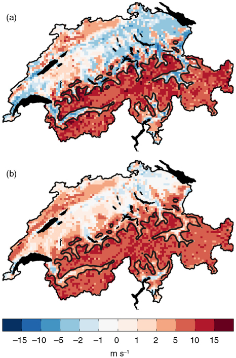
Fig. 13
(a) Differences between the wind gust footprint for ‘Lothar’ based on the COS wind gust estimation method and the wind gust footprint based on the WPD method in m s−1 (i.e. COS – WPD; non-linear colour scheme). (b) Analogous to (a), but shown is the difference between the wind gust speed composite mean for all 84 windstorm events using the COS method and the composite based on the WPD method. The WRF terrain height 1500 m a.s.l. contour line and lakes are outlined.
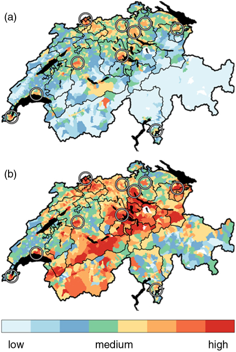
Fig. 14
Composite mean of simulated loss per km2 at municipal level for all 84 windstorm events (colour scheme) using (a) the WPD wind gust estimation and (b) the COS wind gust estimation. Circles indicate the 10 major agglomerations of Switzerland in 2009. Cantonal boundaries and lakes are outlined. Figure 14a is the same as Fig. 9a.