
Fig. 1
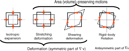
Decomposition of the local motion in 2-D flow. Vectors show the direction of the flow field. This decomposition is complete to the linear order of the Taylor series expansion in eq. (1).
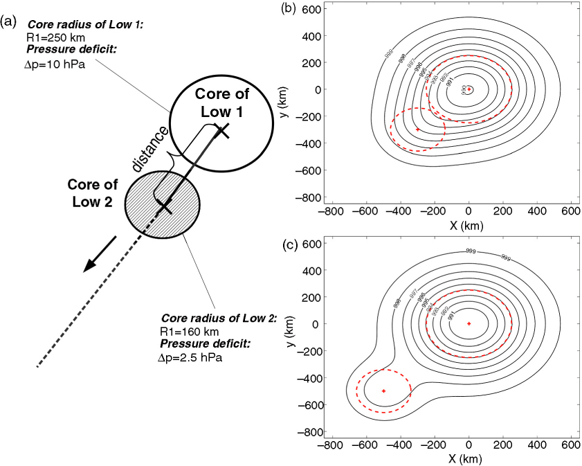
Fig. 2
Experimental set-up of ideal test case 1: the superposition of two low-pressure disturbances with different intensities and sizes on a flat pressure field. The smaller low 2 is moved stepwise along the dashed line following the thick black arrow. (a) Sketch of experimental set-up, (b) pressure field for a distance of 353.6 km, (c) pressure field for a distance of 707.1 km. Red crosses indicate the low centres, red dashed circles correspond to their radii. Domain size: 140×140 grid points; grid resolution: 10 km.
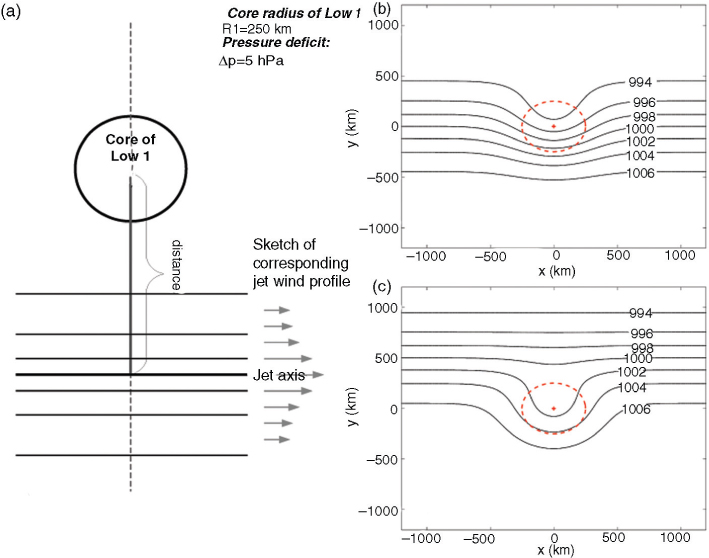
Fig. 3
Experimental set-up of ideal test case 2: the superposition of a low-pressure disturbance and a non-trivial jet streak gradient on a flat pressure field. The jet axis is moved stepwise from south to north as indicated by the dashed lines. (a) Sketch of experimental set-up, (b) pressure field for a distance of 0 km between jet axis and vortex centre, (c) like in (b) for a distance of 500 km (jet axis north of vortex). Red cross/red dashed circles indicate the vortex centre/radius. Domain size: 120×120 grid points; grid resolution: 10 km.
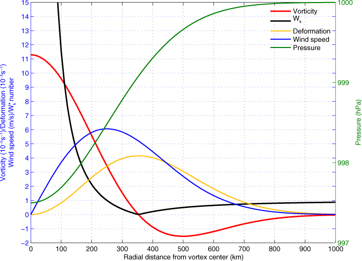
Fig. 4
Undisturbed, axisymmetric reference case: Vorticity ζ(r) in 10−5 s−1, kinematic vorticity number W k (r), deformation (local strain-rate) in 10−5 s−1, wind speed υ(r) in m/s (left axis) and pressure p(r) in hPa (right axis) as function of the distance from the vortex centre. W k =1 at a distance of 250 km and ζ=0 at a distance of 320 km.
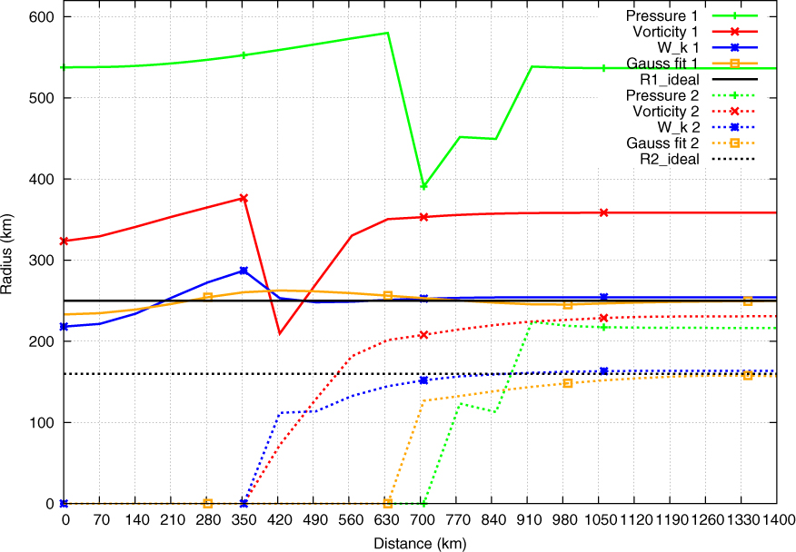
Fig. 5
Identified radii by the four methods in ideal test 1 (superposition of two low-pressure systems 1 and 2). Plotted are the identified radii as a function of the distance between the two centres. Symbols plotted every 5th data point.
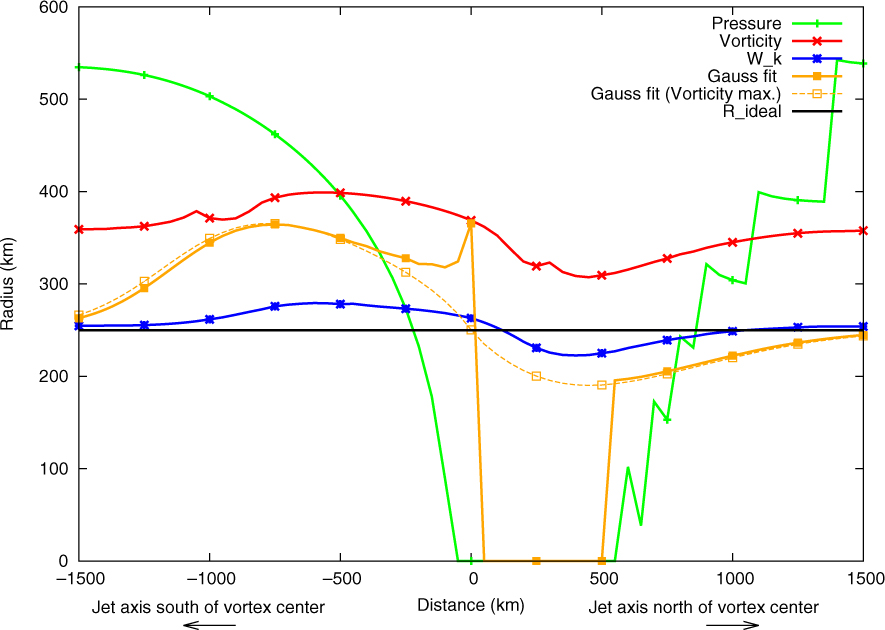
Fig. 6
Radius determination by the four methods of the low-pressure disturbance which was superposed by a jet streak (ideal test 2). Plotted are the identified radii as a function of the distance between the jet axis and the centre of the low (for negative/positive distances the jet axis is south/north of the vortex centre). Symbols plotted every fifth data point. Dashed yellow line: Gaussfit-method applied to the pressure field surrounding the local vorticity maximum instead of the local pressure minimum (solid yellow line).
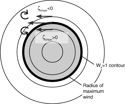
Fig. 7
Scheme of the wind field and shear vorticity of an idealised cyclone (NH). W k =1 contour and radius of maximum wind coincide. Shaded area marks the area of positive shear vorticity (ζshear>0).
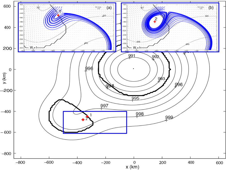
Fig. 8
Streamlines at the vortex core boundary and inside the vortex core: Superposition of two lows with a distance of 636 km between the two centres. Thin black lines are the isobars; bold black lines are the identified W k =1 contour line. The blue box displays the area of the two insets labelled (a) and (b) in the top of the figure. In the insets the streamline patterns (thin blue lines) around two different points are added: (a) Point 1 is located on the W k =1 contour; (b) Point 2 is located inside the W k =1 contour (inside the identified vortex). Grey arrows indicate the velocity vectors around the points 1 and 2, respectively.
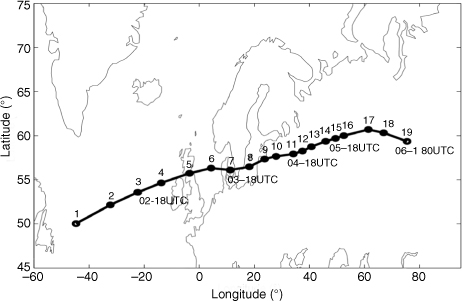
Fig. 9
Track of Anatol's circulation centre in the 1000 hPa level: starting at 2 December 1999 06 UTC. Every circle and number represents a 6-hourly step, some selected dates are additionally plotted below the corresponding circles.
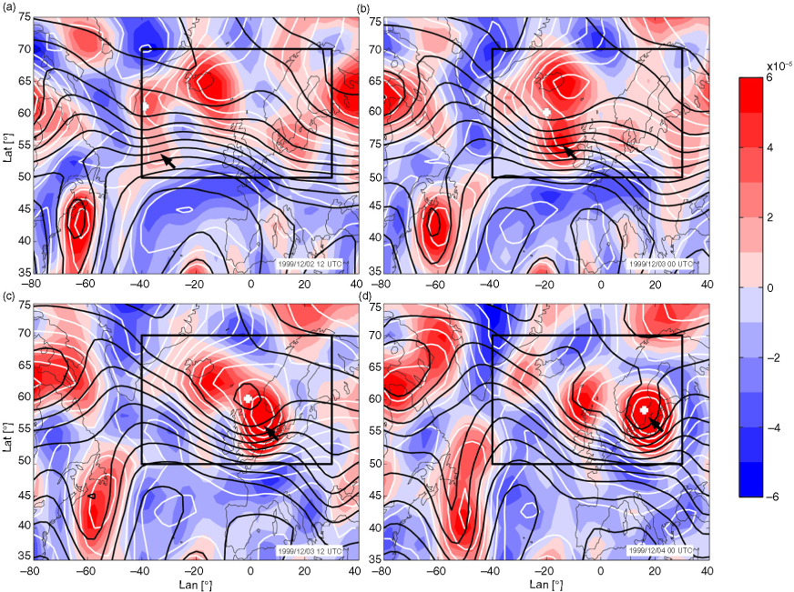
Fig. 10
Development of storm Anatol (2–4 December 1999, 12-hourly steps) in traditional fields: Geopotential height (in gpdm at 1000 hPa (white)/500 hPa (black) contours) and low-level (850 hPa) relative vorticity (colour shaded) fields. Black arrow and white cross indicate the position of the storm centre in 1000 hPa/500 hPa. Contours of the geopotential are given every 4 gpdm in 1000 hPa (white) and every 8 gpdm in 500 hPa (black). Black box corresponds to the section plotted in Fig. 12.
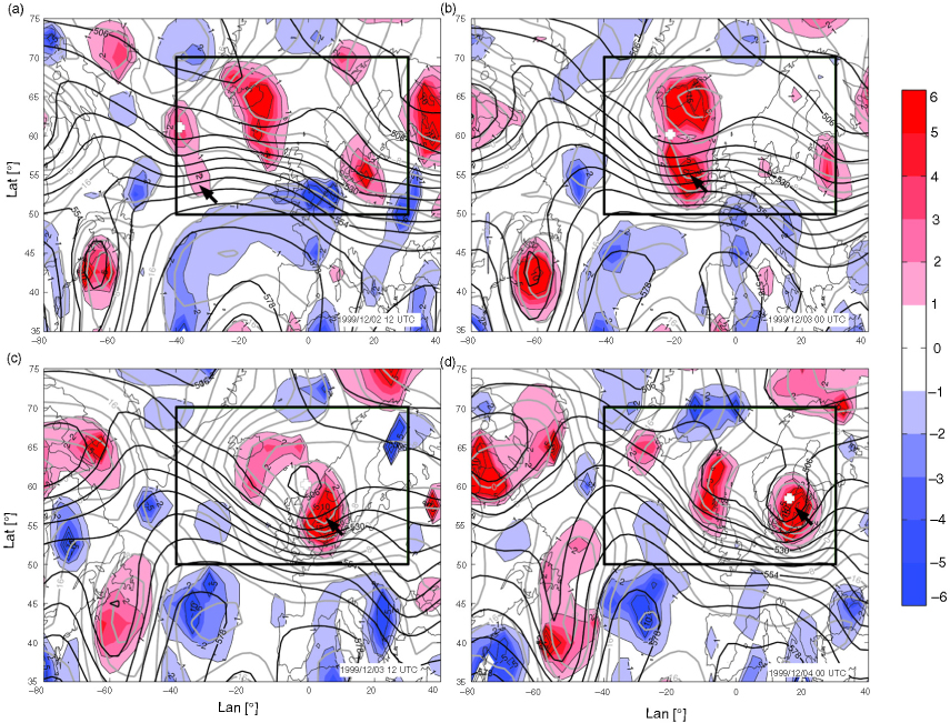
Fig. 11
Development of storm Anatol (2–4 December 1999, 12-hourly steps) in kinematic fields: Low-level (850 hPa) extended kinematic vorticity number (colour shaded) field considering the sign of vorticity. Positive (negative) values of W k correspond to cyclones (anticyclones). Isolines of are added (labelled thin grey contours). Other fields/tokens are similar to that in Fig. 10.
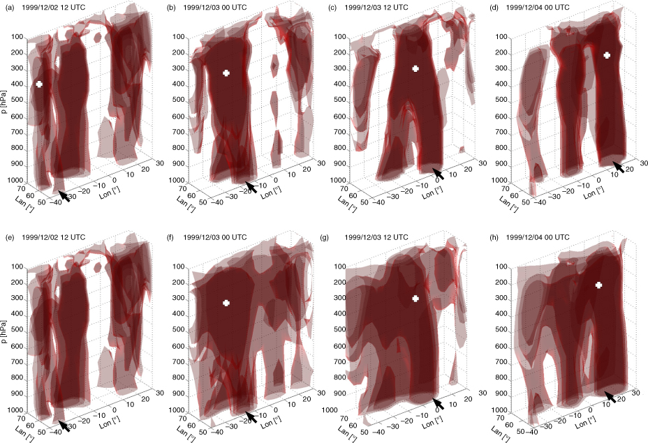
Fig. 12
Vertical development of storm Anatol (2–4 December 1999, 12-hourly steps): in W k (a–d) and ζ g (e–h) fields. Plotted are isosurfaces of the cyclonic (positive) geostrophic vorticity [(1,3,5) 10−5 s−1]: (a–d) Vorticity is plotted in the field of W k >1, (e–h) field of positive geostrophic vorticity. Values of W k <1 as well as negative vorticity values are blank. Lighter colours correspond to lower values of vorticity. Black arrow and white cross indicate the position of the storm centre in 1000 hPa and in the upper levels, respectively.
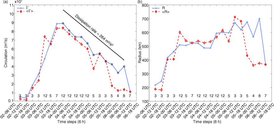
Fig. 13
Properties of storm Anatol over its lifetime: (a) circulation Γ and (b) area A in 6-hourly timesteps starting from 2 December 1999 06 UTC to 6 December 1999 18 UTC; corresponding radius () was added to the right axis in (b). Dashed red lines correspond to the vertical averaged values of Γ and A (small numbers near the bottom indicate the number of vertical levels used for the vertical average), solid blue lines correspond to the value at 1000 hPa. For the calculation of the circulation, geostrophic wind has been used.
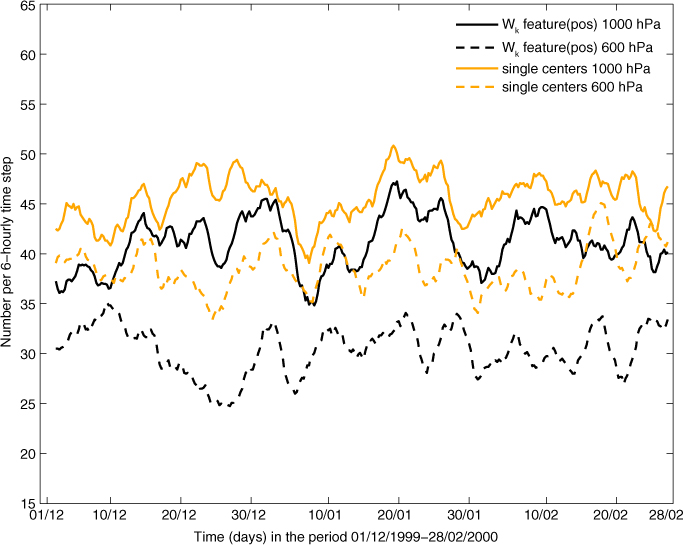
Fig. 14
Three-day running mean of the number of identified lows: cyclonic W k features (black)/single centres (orange) in 1000 hPa (solid) and 600 hPa (dashed) for DJF 1999/2000 in 30°–80° N. Mean numbers/total numbers over the whole period are in 1000 hPa: 41.1/14.339 (W k features), 45.6/15.905 (single centres) and in 600 hPa: 30.4/10.607 (W k features), 38.6/13.469 (single centres), respectively.
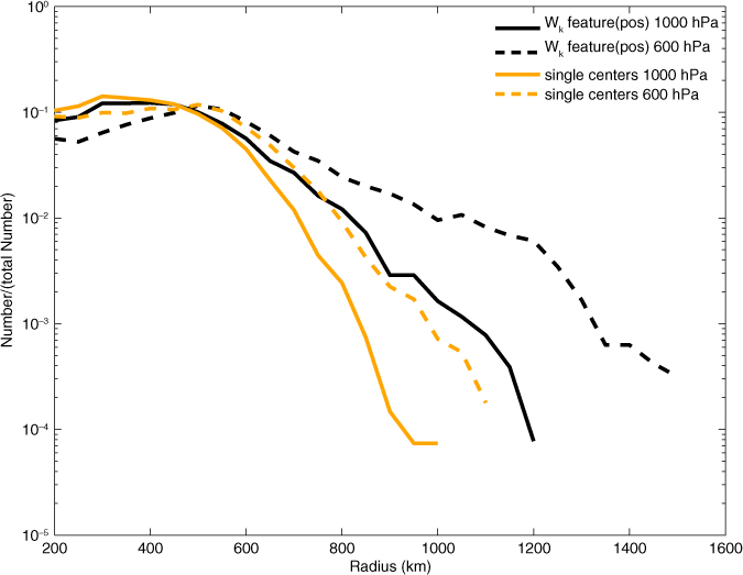
Fig. 15
Relative frequency distributions concerning the radii: cyclonic W k features (black)/single centres (orange) in two different pressure levels (1000 hPa solid, 600 hPa dashed). DJF 1999/2000, 30°–80°N. Only systems with radii ≥200 km were included. Total number of systems in 1000 hPa: 12.862 (W k features), 13.530 (single centres) and in 600 hPa: 9.521 (W k features), 11.148 (single centres), respectively. Note the logarithmic scaling of the ordinate axis.
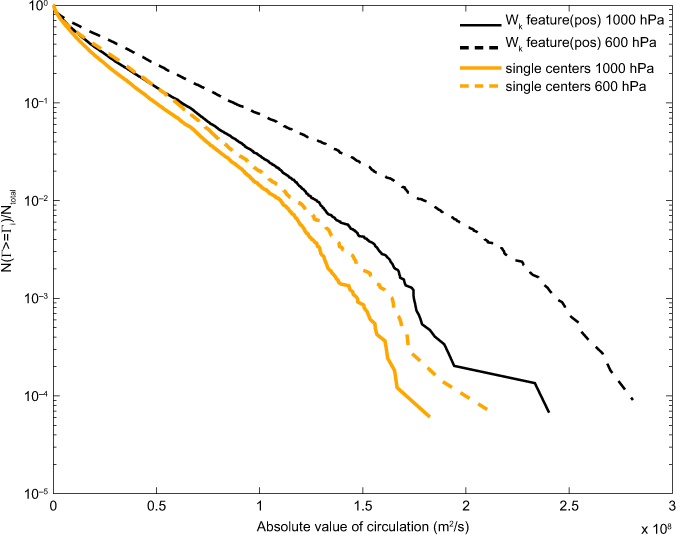
Fig. 16
Complementary cumulative distribution of the circulations: cyclonic W k features (black)/single centres (orange) in two different pressure levels (1000 hPa solid and 600 hPa dashed). DJF 1999/2000, 30°–80°N. Note the logarithmic scaling of the ordinate axis.