
Fig. 1
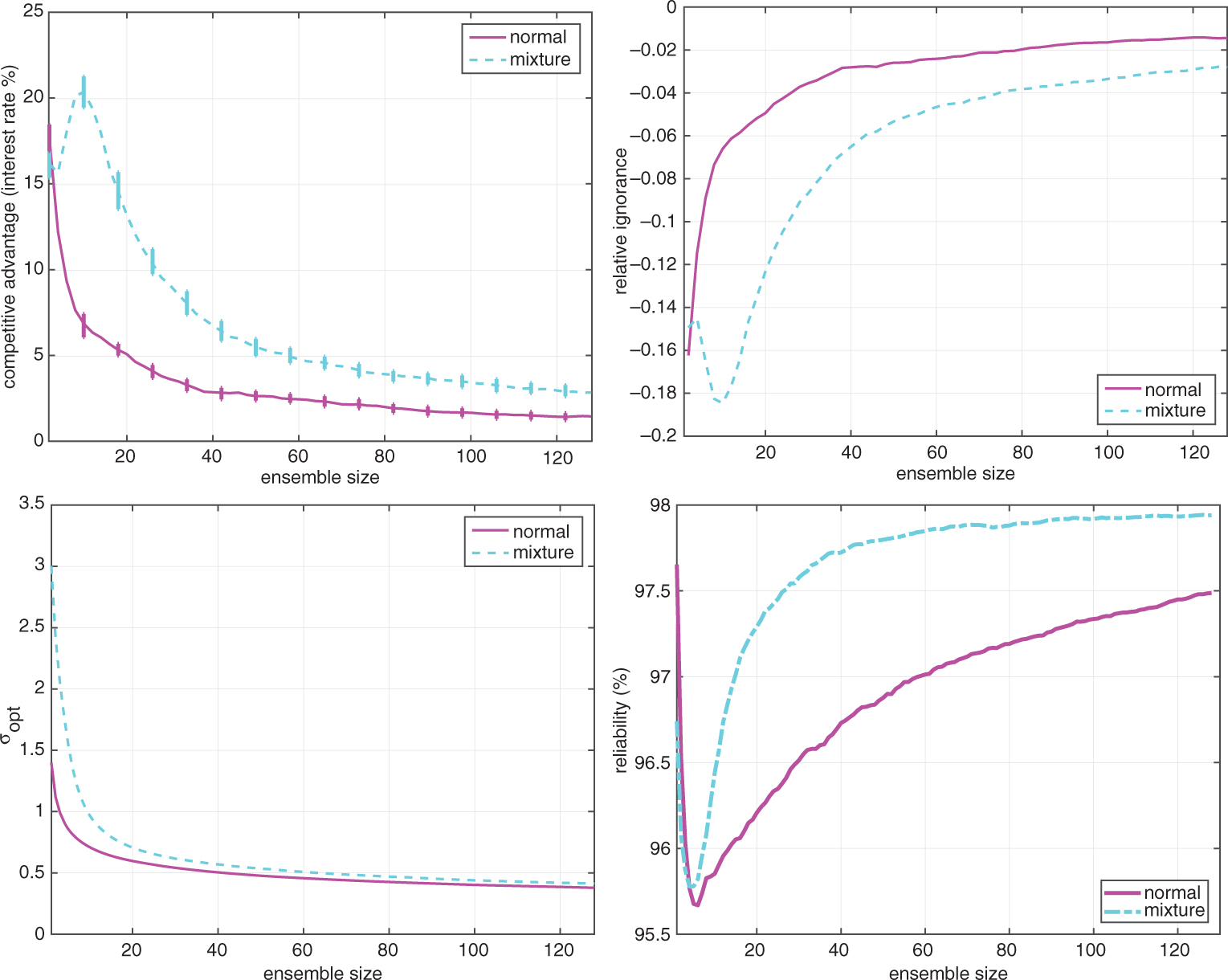
Simple Gaussian and mixture distributions. Top left: Graph of competitive advantage when the ensemble size is doubled as a function of the final ensemble size (shown on the horizontal axis). That is, this is the IGN of an ensemble relative to an ensemble half its size. Top right: Change in IGN when the ensemble size is doubled as a function of the final ensemble size. Note the inverse relationship between competitive advantage and relative ignorance. Bottom left: Graph of kernel width versus ensemble size. Bottom right: Graphs of the reliability PIT as a function of ensemble size. The underlying distributions are the standard normal (solid purple) and a mixture (blue dashed) of normals, π(x), given in eq. (10). For each distribution, at a given ensemble size, the kernel width was chosen to minimise IGN. The bars on the left graphs are the 95 % bootstrap re-sampling intervals. Note that the smallest value of the ensemble size in the above graphs is n=1 (a so-called singleton ensemble).
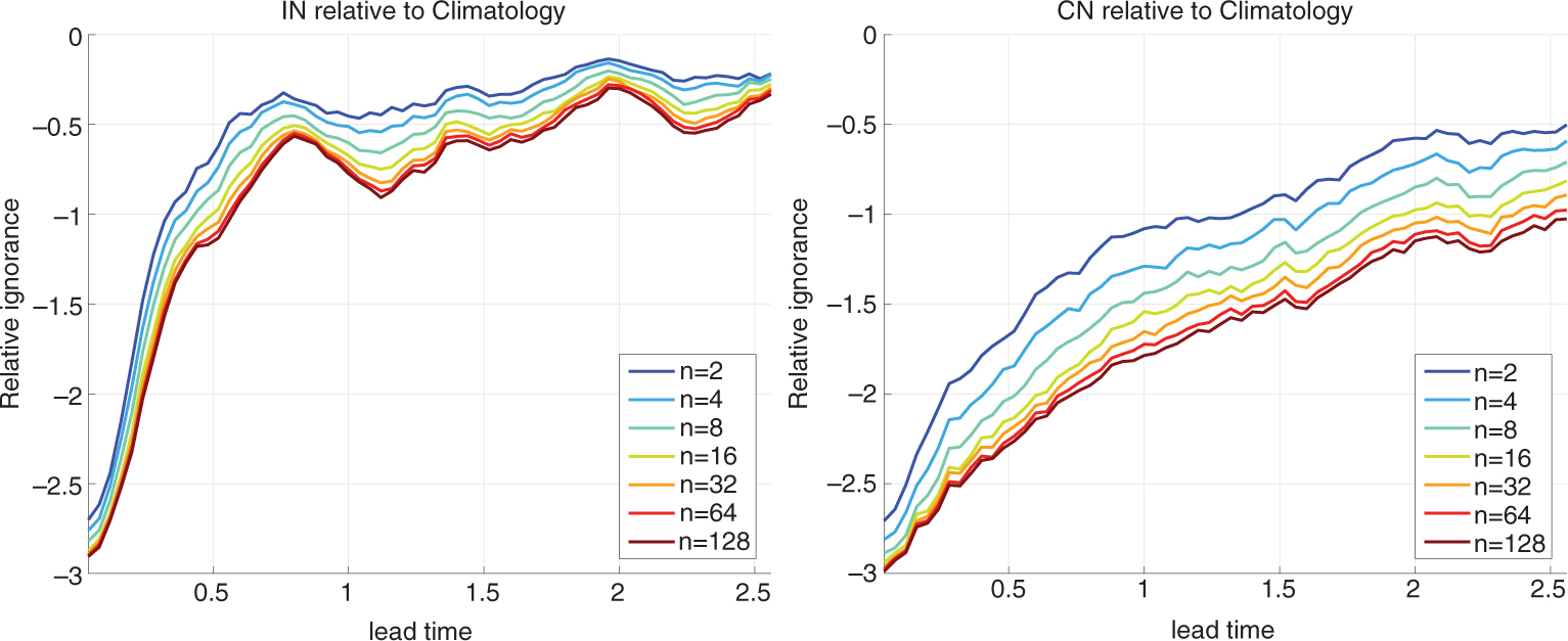
Fig. 2
Moore–Spiegel system. The decay of predictability with time of two forecasts systems of the Moore–Spiegel system. Ignorance relative to climatology is shown as a function of lead time for ensembles of size 2, 4, 8, 16, 32, 64 and 128. Lead-time is reflected by colour. The forecast systems differ in the data assimilation scheme used; Left: The inverse noise (IN) method. Right: The collapsed noise (CN) method. Note the forecast system using CN gives systematically more skilful forecasts. Note that the larger ensembles routinely show greater skill at each lead time for each system.
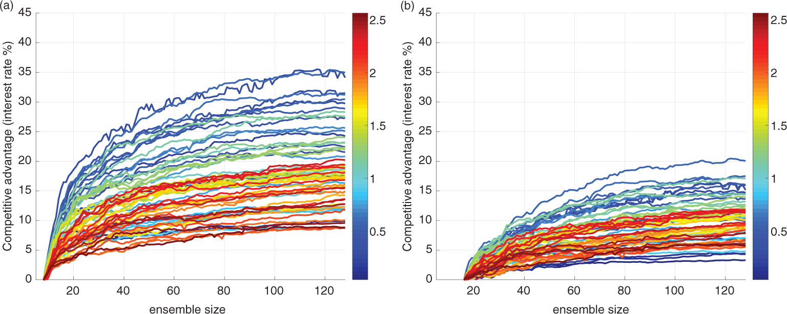
Fig. 3
Moore–Spiegel system with inverse noise. Graphs of competitive advantage when increasing the ensemble size relative to a reference ensemble size. Left: Reference ensemble-size is 8. Right: Reference ensemble-size is 16. The colour bars indicate lead time. Note that when the competitive advantage is sloping upward towards the right-hand side of each graph, the benefit of increasing the ensemble size is still increasing at the largest ensembles tested. At shorter lead times (dark blue) the benefit tends to be greater than longer lead times (dark red).
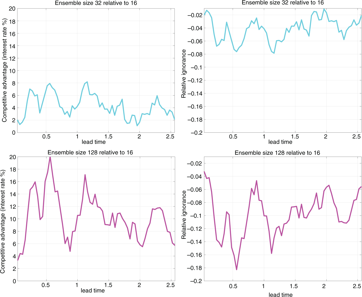
Fig. 4
Moore–Spiegel system with inverse noise. The two graphs on the left show the competitive advantage as a function of lead-time for an ensemble size of 32 relative to 16 as a functions of lead-time (top) and 128 relative to 16 (bottom). Each curve corresponds to a slice through Fig. 3. The IGN scores for the same comparisons are shown on the right. Note the symmetry between ignorance and competitive advantage [flipping over (y → −y) in a graph in the right column leads yields the pattern of a curve on the left].
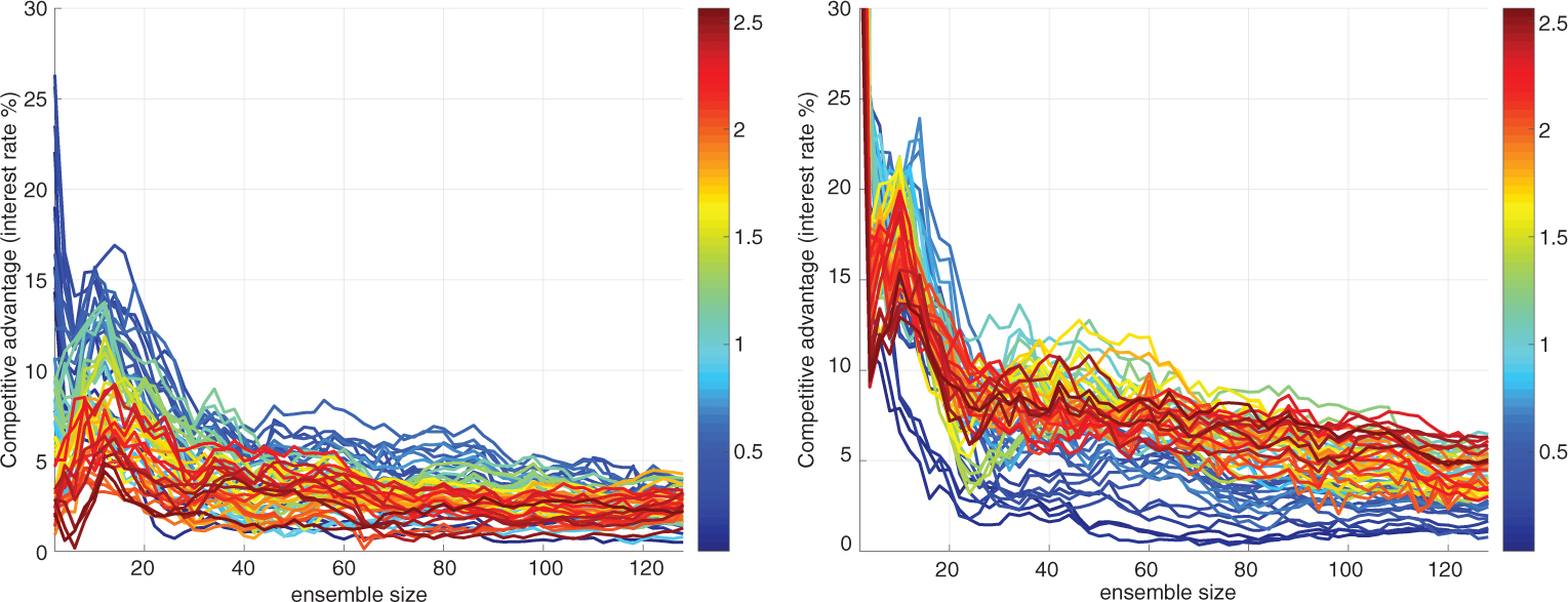
Fig. 5
Doubling the ensemble size in the Moore–Spiegel system. Left: Graphs of competitive advantage gained by doubling the ensemble size of IN forecast systems as a function of the final ensemble size. Right: Graphs of competitive advantage gained by doubling the ensemble size of CN forecast systems as a function of the final ensemble size. Each line on a given graph corresponds to the forecast lead time according to the corresponding colour bar. Note that doubling the ensemble size is demonstrably beneficial at all lead times, and the (more expensive) CN-based forecast systems tend to benefit more than the IN-based systems, especially at longer lead times.
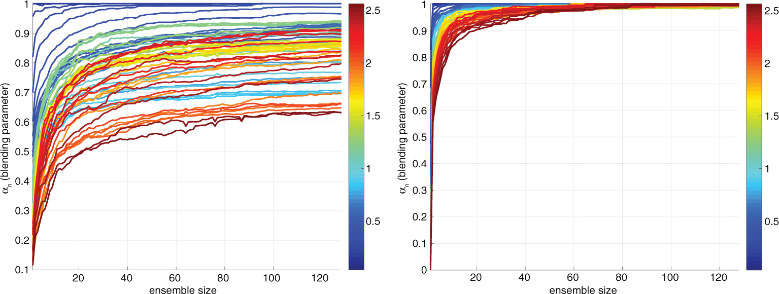
Fig. 6
Moore–Spiegel system. Graphs of blending parameter (α n ) versus ensemble size determined by minimising the average ignorance score over a forecast–outcome archive. Left: IN-based forecast systems. Right: CN-based forecast systems. Note the systematic increase of α n with ensemble size in each panel. The colour bars on the right of each panel correspond to lead time.
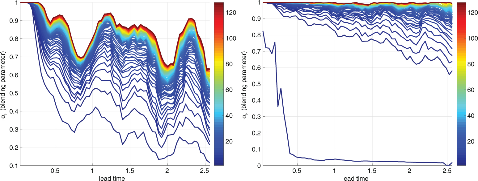
Fig. 7
Moore–Spiegel system. Graphs of blending parameter (α n ) versus lead time under each of the two data assimilation strategies. Left: IN-based forecast systems. Right: CN-based forecast systems. In the IN-based systems the general decrease in α n with lead-time is rather complex; nevertheless the value of α n for these systems is systematically lower than that for the CN-based systems, and thus the weight on climatology is significantly greater. In the CN-based forecast systems, the decrease is more regular; interestingly at a given lead-time the value of α n is greater for the larger lead-times. This suggests a potentially resolvable shortcoming in the CN data assimilation scheme. The colour bar on the right-hand side of each graph indicates the number of ensemble members.
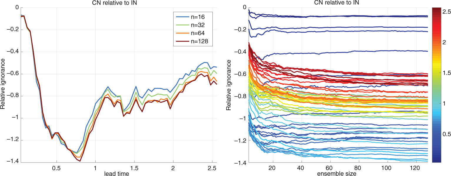
Fig. 8
Contrasting skill due to data assimilation scheme: Moore–Spiegel system. The skill of competing forecast systems which differ only in the data assimilation scheme is contrasted in the Moore–Spiegel system: each panel shows IGN of CN-based forecasts relative to those of IN-based forecasts, thus negative values imply more skill in the CN method. Note that all values are negative. Left: Ignorance as a function of lead time for four ensemble sizes (16, 32, 64 and 128). Note that the forecast system using CN gains additional skill above the one using IN as the ensemble size increases. Right: Ignorance as a function of ensemble size for a variety of lead times (as indicated by the colour bar on the right-hand side of the panel). Note that the benefit of using CN is greatest in the medium range, lead times between 0.5 and 0.9; while the advantage continues to exceed half a bit (a 40 % gain in probability, on average) at longer lead times, it is less than a tenth of a bit at short lead times. This suggests that the CN data assimilation might require improvement (to justify its added cost) if the focus is on shorter lead times. Also note in the right panel that for longer lead times (reddish) the skill curves are still sloping down even at the largest ensembles tested, indicating that the CN-based forecasts are improving faster as the ensemble size is increased even at the largest ensembles tested.
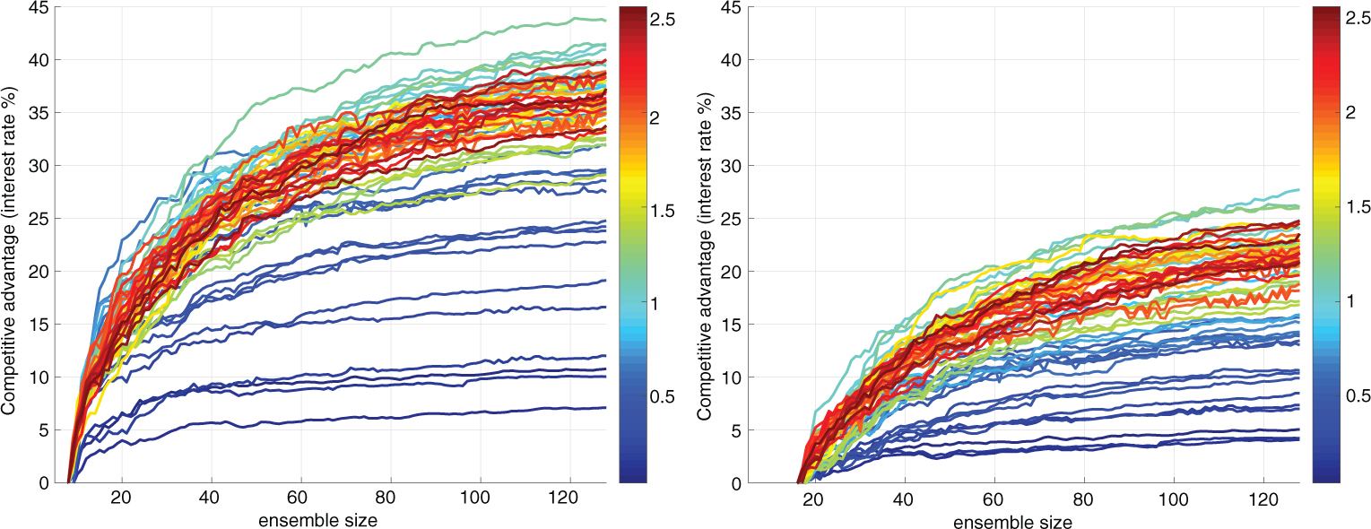
Fig. 9
Moore–Spiegel system with collapsed noise. Graphs of competitive advantage when increasing the ensemble size relative to a reference ensemble-size. Left: Reference ensemble-size is 8. Right: Reference ensemble-size is 16. Contrasting this figure with its counterpart (Fig. 3) suggests that for all but the shortest lead times, using the CN algorithm increases the gain obtained by these increases in ensemble size. The colour bar on the right-hand side of each graph indicates the lead time.
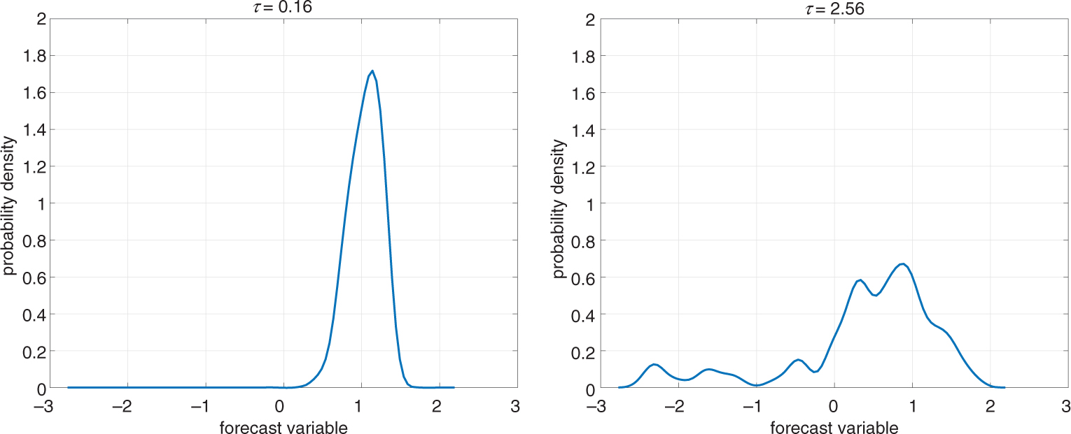
Fig. 10
Moore–Spiegel with collapsed noise. Two illustrative forecast distributions corresponding to the same initial ensemble; the ensemble size n=128. The left panel at lead time τ=0.16 shows a distribution that might be well described as normally distributed. The right panel, at longer lead time τ=2.56, would be less well described by a normal distribution.
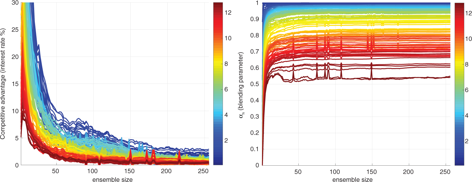
Fig. 11
Circuit with inverse noise. Left: Graphs of competitive advantage of an ensemble versus an ensemble half its size. All forecast results in this article are out of sample. Right: Graphs of blending parameter versus ensemble size, note that α n saturated (the curve goes flat) at smaller ensemble sizes than in the case of IN-based forecasts of Moore–Spiegel. Each line on a given graph corresponds to the forecast lead time according to the corresponding colour bar.
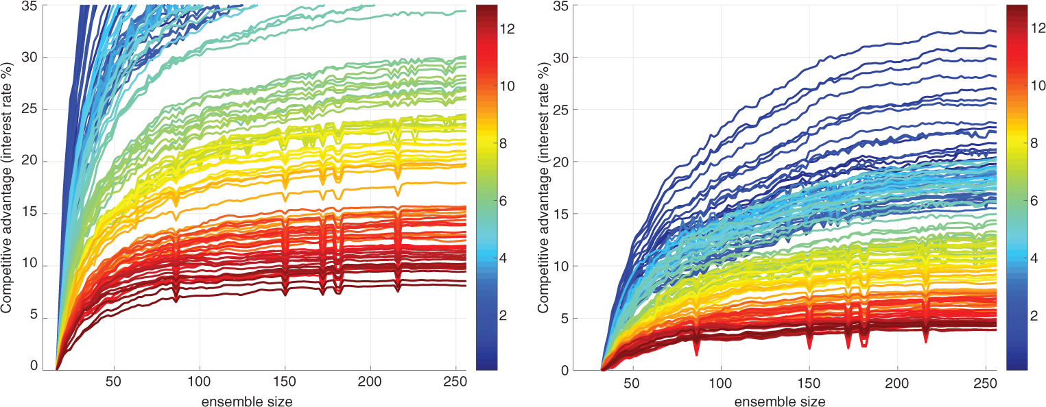
Fig. 12
Circuit with inverse noise. Graphs of competitive advantage when increasing the ensemble size relative to a reference ensemble-size. Left: Reference ensemble-size is 8. Right: Reference ensemble-size is 16. The colour bars indicate lead time. Note that when the competitive advantage is sloping upward towards the right-hand side of each graph, the benefit of increasing the ensemble size is still increasing at the largest ensembles tested. At shorter lead times (dark blue) the benefit tends to be more than longer lead times (dark red). The colour bar on the right-hand side of each graph indicates the lead time. The occasional glitches (short, sharp drop-outs of low skill) are due to a well understood flaw in our automated kernel-selection algorithm.
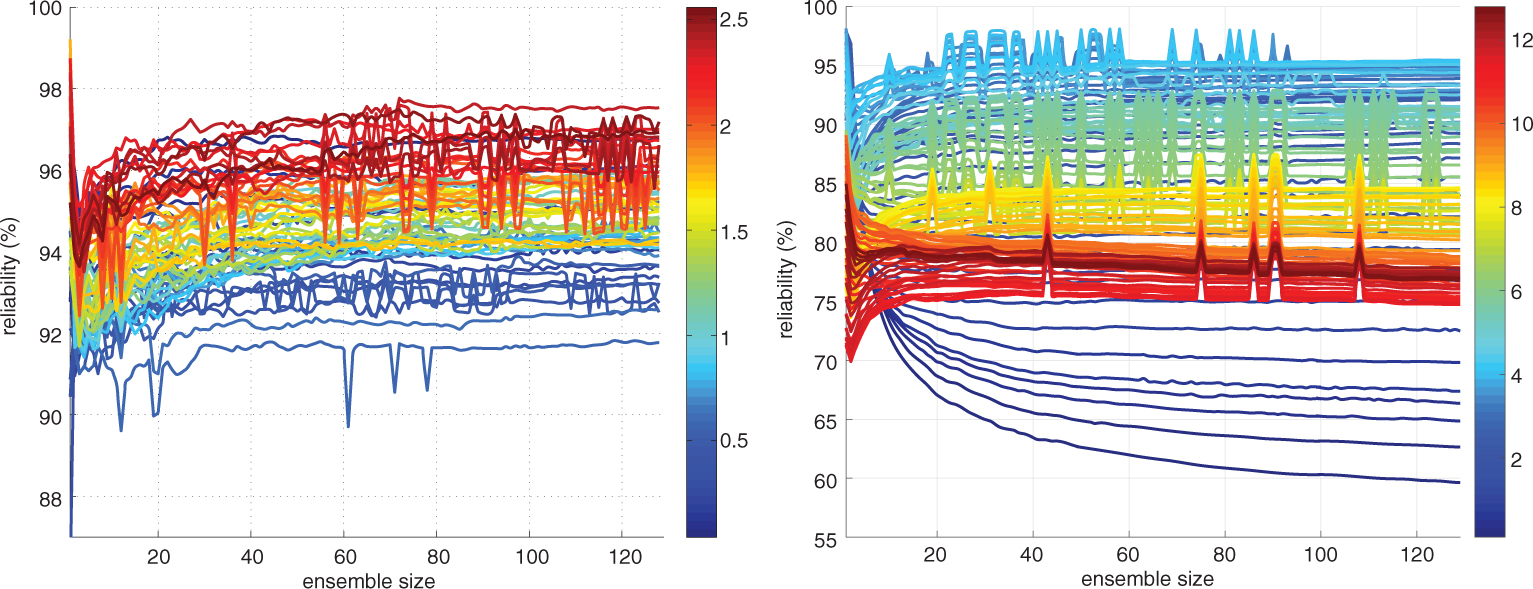
Fig. 13
Quantifying reliability PIT . Graphs of reliability PIT as a function of ensemble size. Left: Moore–Spiegel system under CN-based forecast systems. Right: Circuit under IN-based Forecast systems. Here forecasts of the circuit, for which the model is imperfect, display two qualitative differences from the Moore–Spiegel system and the mixture distributions shown in Fig. 1. First, at the shortest lead times (dark blue) reliability PIT decreases significantly with ensemble size. Second, at the longest lead times (orange and red) there is a slow decrease in reliability PIT rather than a plateau. The occasional glitches are due to a well understood flaw in our automated kernel selection algorithm.
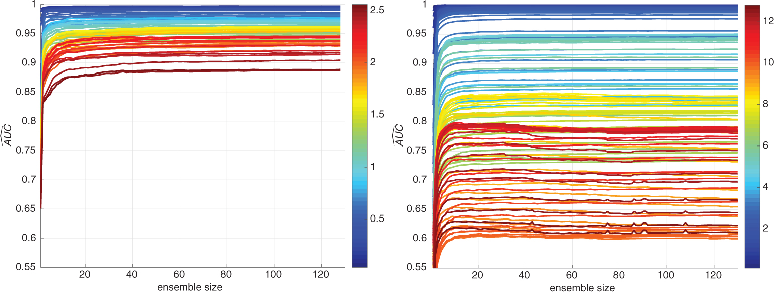
Fig. 14
Resolution ROC . Left: Graphs of the area under the ROC curve , resolution ROC , which is considered a measure of resolution. Left: For the Moore–Spiegel system under CN-based forecast systems. Right: For the Circuit under IN-based forecast systems. The colour bar on the right-hand side indicates the forecast lead time.
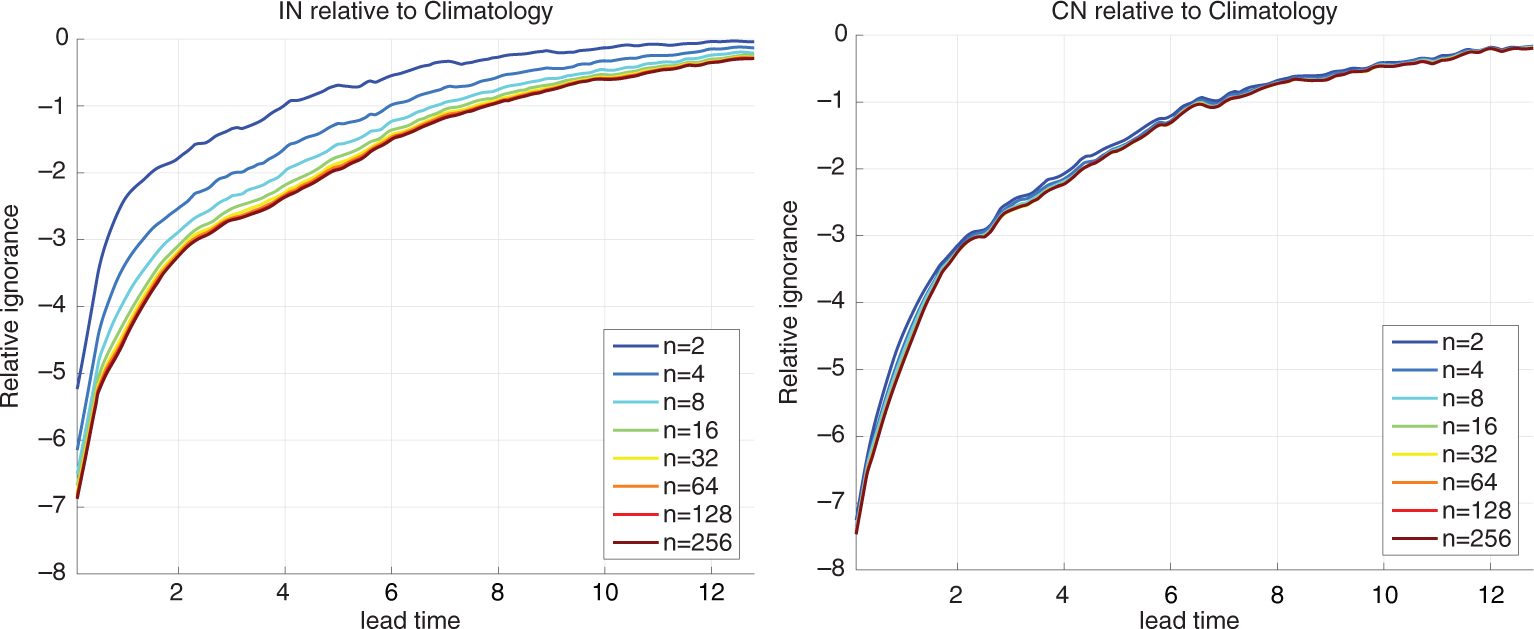
Fig. 15
Decay of predictability of the circuit in two forecast systems based on different data assimilation schemes. IGN score of forecasts of the circuit relative to climatology for eight ensemble sizes. The two forecast systems use different data assimilation methods. Left: A inverse noise (IN)-based forecast system. Right: Collapsed noise (CN)-based forecast system, with an assimilation window of two steps. Note that the gain from merely moving from an IN-based forecast system to a CN-based forecast system alone is much greater than the gain from increasing the ensemble size by a factor of 128 in the IN-based forecast system.